| By Louis-Charles Généreux and Allen Xu |
Problem definition
As avid sports fans, we have always been intrigued by the opaque world of player evaluation. In sports like ice-hockey, where teams’ salary spending is capped, signing the right players, at the right price is essential to attaining team success. With most National Hockey League (NHL) teams spending close to all the money available under the salary cap, a team’s competitive edge comes partly from its ability to identify “under-priced” players. General Managers’ (GMs) responsibility is to build rosters of high-performing, fairly-paid players to maximize their team’s chances of success. In 2021, the NHL salary cap is $81.5M, meaning that no team can see its total player compensation exceeding this figure; see the NHL’s statement and a brief explanation of the cap’s history.
Because hockey is a non-static sport, with continuous flow, statistical analysis is not as straightforward as it is for baseball (where there are binary outcomes for each play). GMs are often retired players, who rely more on subjective reports from a vast network of scouts than on data to make contractual decisions, creating biased decisions. Research by Lanoue (2015) at the University of Windsor has identified player attributes or variables that translate to salary premiums, with all other factors being held constant. For example, being a past Stanley Cup winner typically translates to a 19% salary premium, while being an enforcer (a player who engages in on-ice fist fights) leads to a 15% salary premium; these highly-priced attributes might not actually translate to team success.
Acknowledging that GMs have biases that lead them to paying salary premiums to players who might not be the highest performers on their teams, we wondered: are these premiums worth it? To answer this question we set out on a mission to determine each NHL players’ fair salary, or what each player should be paid based on his contribution to his team’s success. In doing so, we:
- Built a tool to evaluate each player’s performance based on team contribution metrics
- Clustered players based on said metrics and calculated within-cluster average salaries for comparable players
- Developed a framework to assess General Managers’ effectiveness based on tendencies to over/under pay players relative to their contribution
Before discussing our approach and findings in more details, we recommend that readers not familiar with the game of ice hockey watch the following short video. It succinctly explains the rules of the game while also showing game footage.
Sources of inspiration for this project
Sports Analytics have become a hot topic in the last decades, especially after the public witnessed the success of analytics departments in professional sports, highlighted by the movie Moneyball (based on Michael Lewis’ best-seller). As previously mentioned, hockey is a continuous sport, making it more difficult to model statistically. However, many researchers and fans have published papers on the sport. While our research may not be fully exhaustive, we are fascinated by the work published by Ryder (2012), Gramacy (2013) and Lanoue (2015) and by statistics released on analytics websites such as Evolving Hockey. Below is a short summary of their findings and a discussion on how we intend to build on some of their work.
Historically, one of the most common metrics used in the field of hockey player evaluation has been plus-minus (the absolute goal difference between goals for and against while a player is on the ice). While this metric is simple and does not require granular play-by-play data to be computed, Gramacy (2013) points out that this traditional evaluation metric is largely dependent on the performance and strength of the whole team instead of individual players. The same can be said of other shot-based metrics such as Fenwick and Corsi.
Ryder (2012) proposed the idea of marginal contribution, or crediting each goal and assist for a team to individual players with different weights based on factors like points produced, plus-minus, the strength of the opposing team and play situations. We believe this paper to be a major breakthrough in the hockey analytics space: Ryder attributed shares of each of a team’s goals (for and against) to players on the team, allowing his readers to compare offensive contribution with defensive liability. More recently, websites like Evolving Hockey have created some buzz in the hockey community with the publication of their Goal Above Replacement (GAR) metric, which aims to measure whether a player performs above “replacement level”.
Beyond the evaluation of player contribution, another common theme in prior research has been to determine whether or not players are economically valuable based on their contracts. Lanoue (2015) studied the relationship between winning a Stanley Cup and contract terms for players. Gramacy (2013) clustered players based on their position and created a probability density function based on performance across different salary brackets.
In this paper, we aim to highlight both offensive and defensive prowess of each player, but with more granularity than Ryder. Rather than base our analyses on season-long aggregated goals and assists data like Ryder (who computed metrics based on one row of summary statistics per player), we will build our metrics based on shot attempts and with many more nuances such as shot location, difficulty and context (thanks to the availability of play by play statistics). Building metrics using shot attempts rather than goals also allows us to compute expected goals, which can be compared with actual goals scored. This will allow us to explore the notion of “clutch” play or conversion of opportunities in this paper. We will then perform player clustering, taking into more dimensions than Gramacy, such as career stage, position, playing style and physicality of the players. Finally, we will evaluate GMs’ dealmaking abilities, which has not yet been attempted in quantitative fashion.
Analysis
Development of player evaluation metrics
To evaluate players’ performance, we analyzed each scoring opportunity of the 2019-2020 and computed new player evaluation metrics, taking shot difficulty and play situation into account. The metrics we developed provide more context into player contribution than simple statistics such as scoring related metrics (e.g., goals or assists produced, plus-minus), which are partially driven by luck and overall team strength. Compiling the number of opportunities created and assessing their likelihood of conversion to goals requires play-by-play breakdowns of games; more specifically we need to know which players were on the ice for each shot taken and what was the location of the shot relative to the opposing team’s net.
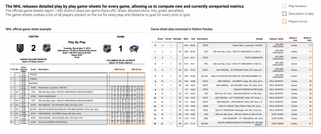
We obtained our detailed game data from the NHL’s official game-sheets, which report ~300 distinct plays per game (face-offs, shots, blocked shots, hits, goals, penalties). The game-sheets contain a list of all players present on the ice for every play, in addition to distance to goal for every shot or goal. In Figure 1, we show an official game sheet and the extracted data in pandas format after scraping. Play by play data for this project consists of:
- Play description (shot, goal, face-off, shot block, play stop)
- Distance from net, X and Y coordinates of a play
- Strength (even strength: both teams have 5 players on the ice, power-play/penalty-kill: a team has a 1 man advantage due to a penalty)
- Name of all players on the ice for a play
While all of these fields can be extracted from scraping of game-sheets (as displayed in Figure 1), they can also be extracted with a bit of data cleansing using the various tables in the following data set (https://www.kaggle.com/martinellis/nhl-game-data).
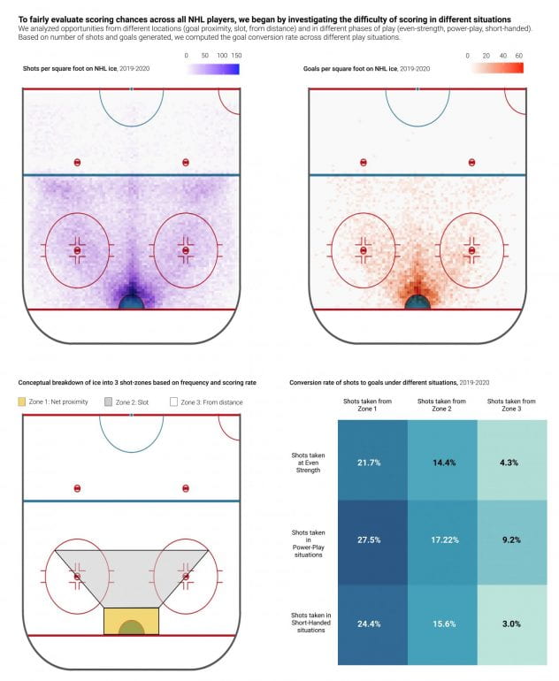
With data on each shot taken during the 2019-2020 NHL campaign, we computed the expected % conversion of shots to goals, based on shot location and play situation. More specifically, we split the offensive zone in three zones:
- Zone 1: Net proximity
- Zone 2: Slot (good angle to net and reasonable distance to net)
- Zone 3: All other shots taken
We then segmented all shots taken based on three possible game situations:
- Even Strength: Both teams are playing with equal numbers of players
- Power-Play: The attacking team (the team taking the shot) has a one or more men advantage thanks to penalties taken by opposing players
- Short-Handed: The attacking team (the team taking the shot) is short one or more men due to a penalty taken by a team mate
In Figure 2, we present 4 images:
- On the top left, we show a heat map of shots per square foot in the NHL offensive zone during the 2019-2020 season. We see heavy shot volumes around the net and a reverse triangle (in zones where the shot angle to the net is advantageous)
- On the top right, we show a heat map of goals scored per square foot in the NHL offensive zone during the 2019-2020 season. We see heavy goal volume in close proximity to the net, but minimal goals from elsewhere (indicating that conversion rates is not equal across the ice)
- On the bottom left, we split the NHL ice in 3 zones, which we will use for our analysis (net proximity, slot, from distance)
- On the bottom right, we compute the conversion rate of shots to goals based on shot zone (from the bottom left figure) and the game situation (even strength, power-play, short-handed)
These analyses confirmed general knowledge that:
- the conversion rate of shots to goals is generally higher as distance to goal is reduced and
- the conversion rate of shots from a given zone is higher in power-play situations
To compute player specific metrics, we first summarized all shots taken and all shots given to the opposing team while a player is on the ice, for each player-game combination during the 2019-2020 season (resulting in 40,000+ player-game entries). Based on this information and on the shot conversion rates displayed in figure 2, we began computing a set of new metrics:
(1) Expected goals for and against, generated while player is on the ice:
- Expected goals contributed to: the summation of (total number of shots taken by team while player is on the ice per zone-situation * shot conversion rate)
- Expected goals given: the summation of (total number of shots taken by the opposing team while player is on the ice per zone-situation * shot conversion rate)
These metrics were then normalized per 60 minutes played for each player, allowing for “apples to apples” comparison across players. For interpretation purposes, it is expected that players with high “expected goals contributed to” generate high number of scoring chances for their teams, while players with high “expected goals given” are defensive liabilities (they give up many scoring chances to opponents).
(2) Offensive contribution to defensive liability ratio:
- Expected goals contributed to / Expected goals given: the ratio of “expected goals contributed to” and “expected goals given”
A number above 1 indicates that the player generates more offensive chances than he gives up (positive contributor to the team).
(3) Player-specific ability to convert chances to points:
- Clutch factor: Actual points produced (goals + assists) divided by expected goals contributed to
A high number can indicate “clutch” play, an ability to perform under pressure, or pure luck (leading to higher conversion). A low “clutch factor” indicates that a player converts opportunities to points at a lower rate than peers, all other factors considered.
We believe these metrics offer a much more telling story on actual player contribution than traditional NHL statistics. Traditional metrics, which are purely outcome driven are influenced by luck, team strength and do not factor in play difficulty or situational details. On the other hand, our new metrics allow us to see discrepancies between expected and actual offensive production, but also gain insight into a player’s defensive liability (which traditionally go un-measured and un-reported). In Figure 3, we provide a definition and interpretation for these new metrics and show sample player profiles.

To highlight the potential value of our new player evaluation metrics to NHL executives, we studied the profile of two 2019-2020 standouts who both were elite point-scorers, but had completely different “clutch factors”. For instance Bo Horvat, whose calculated “expected total goals contributed to” was 81.5, produced 53 points (22 goals and 31 assists). Mika Zibanejad, whose “expected goals contributed” was 69.2, produced 75 points (41 goals and 34 assists). Full player profiles for these two players are provided in Figure 4.
While fans and executives might jump to conclusions that Zibanejad is far superior to Horvat based on traditional statistics (22 more points produced over the season), the use of “expected goals contributed to” and “clutch factor” tells a more complete story.
Horvat managed to produce a first-tier offensive output with 53 points while being on the NHL’s low end of the clutch factor range (one might say that he had bad luck). Zibanejad, on the other hand was among the players with the highest “clutch factor” in the whole league, indicating that he certainly benefited from lucky bounces throughout the campaign. On the long run, we suspect that luck might display some mean-reverting behavior.

Player clustering and evaluation of fair salary
After having developed new metrics to compare players more fairly, we set out to cluster players in order to find “fair salaries” within each cluster. The dimensions used to cluster players were the following:
- Net contribution per 60 minutes: the difference between goals contributed per 60 minutes and goals given per 60 minutes
- Offensive skills: based on scaled expected goals contributed per 60 minutes
- Physicality: based on scaled number of hits during the full season
- Position: forward or defense-man
- Career stage: veteran player (28 and older) or young player (27 and younger)
In Figure 5, we illustrate the full clustering and present some notable NHL stars who fit in each cluster.
At the highest level, all 671 regular NHL players from the 2019-2020 season can be split into those whose net contribution is positive (those who generate more scoring chances than they give up) or those whose net contribution is negative. We can then split these two groups again based on their offensive skills (those who generate above average offensive chances per 60 minutes played, versus those who don’t). Interestingly, it is possible for players to be offensive-threats but overall liabilities for their teams. It is also possible to not be offensive threats (i.e., produce less offense per 60 minutes than average NHLers) but be net positive contributors to the team.
For example, some high-end offensively-skilled players such as Sam Bennett or Bobby Ryan (negative net contribution players, who are offensive threats) generate more scoring chances per 60 minutes than their peers, yet are overall negative contributors to their teams… the quality chances they give up to opponents outweigh the scoring chances they generate! On the flip side, veterans such as Tyler Bozak and Derek Stepan (positive net contribution, all-rounders who do not figure within the league’s scoring elite) are not flashy offensively but are highly effective; they give up less chances to opponents than they produce for their teams.
Running this clustering exercise allows us to identify value-adding players (positive net contributors) and the true elite of the NHL (positive net contributors, with high offensive skills: those who create high numbers of offensive opportunities). This clustering was not based on traditional output-based statistics, but rather on the quality of chances created and on the overall net contribution of players (taking into account the defensive aspect of the game). To determine fair salaries within a cluster, we make the assumption that based on their high similarities in performance metrics, players who are within a given cluster are comparable. We averaged the salary of all players within a cluster to estimate the “cluster fair salary”, for each player archetype. We see a few trends:
- For equivalent profiles (similar net contribution, offensive skills, physicality and position), veterans tend to be paid more than younger players. This is partly due to the fact that NHL entry level salaries are capped for the first 3 years of players’ careers).
- On average, positive net-contribution players are better remunerated than negative net-contribution players.
- Offensive threat, positive net-contribution players (the NHL’s real elite) are the highest remunerated.
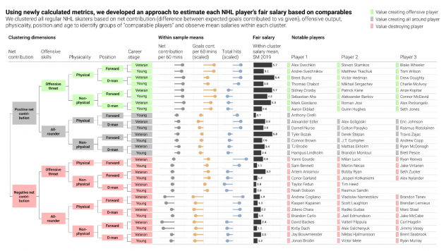
Figure 5: Clustering of NHL players and evaluation of fair-salary within each cluster
Assessment of General Manager effectiveness
After having computed each player’s fair salary based on clustering, we set out to evaluate GM effectiveness. Our objective was to determine whether or not a GM has a tendency to over or under pay his players (relative to their fair salary).
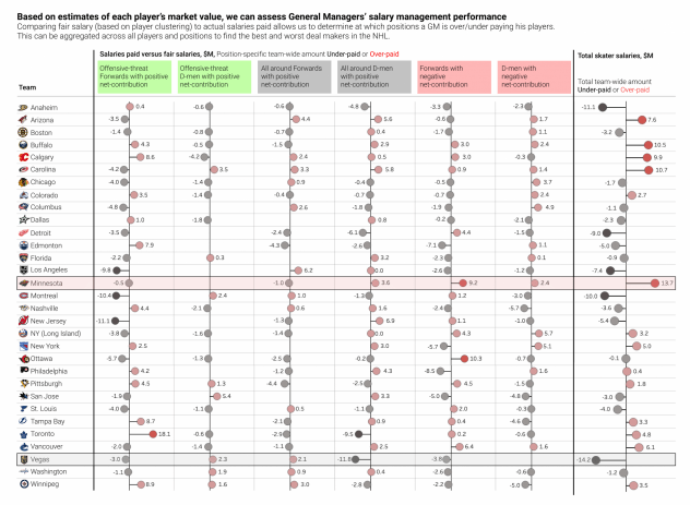
The first step to running this analysis is assigning all NHL players to their respective teams and aggregated archetypes as displayed below in Figure 6. All players under contract by a given team and GM are classified based on their cluster, and are represented by a dot colored based on the comparison of their actual salary to their fair salary.

After assigning players to their teams and simplified cluster, we summed up the difference between total salaries paid and total fair-salaries for a given team and simplified cluster We summed the over/under-spend amount across all clusters to determine the team-wide amount saved or over-spent, relative to fair salaries. The amount over/under-spent by a team for a given archetype is displayed in Figure 7.
During the 2019-2020 season, the Minnesota Wild franchise overpaid its players by 13.7M relative to their players’ performance while the Vegas Golden Knights under-paid their players by 14.2M
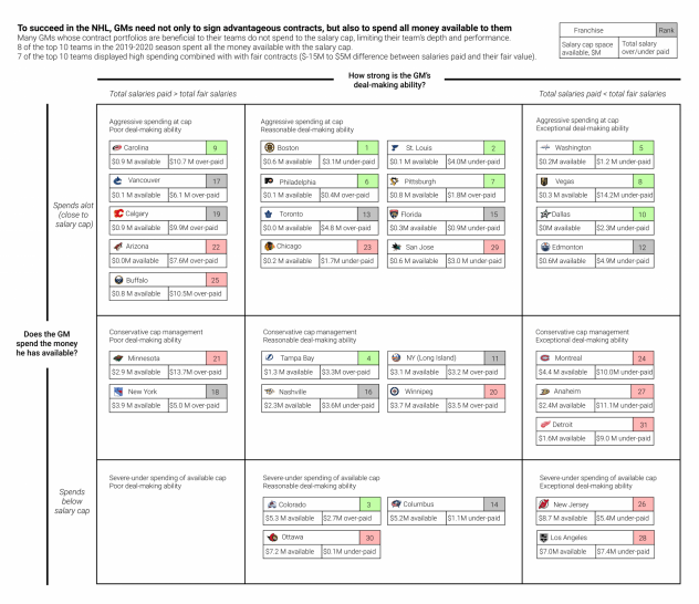
In closing, we mapped each NHL team based on two key GM characteristics:
- To what extent does the GM spend the money available to him (how much money below the salary cap is left at the end of the season)?
- How strong is the GM’s deal making ability (does he tend to over/under spend on player salaries versus their fair salaries)?
In doing so, we discovered that signing advantageous contracts is not enough to guarantee success in the NHL; winning GMs sign better contract deals than their peers, but also spend more in absolute terms. GMs who have constructed successful teams in 2019-2020 have spent close to all money available under the salary cap ($81.5M maximum), resulting in very deep teams. For example in Figure 8, we see that:
- 8 of the top 10 teams in the 2019-2020 season spent all the money available under the salary cap.
- 7 of the top 10 teams displayed both high spending on salaries combined with fair contracts (paying players what they should be paid).
Conclusion and discussion on possible future improvements
As we discussed in our short literature review, many have ventured into advanced player evaluation and forecasting of fair salaries for NHL players. We believe that we have made new contributions to the hockey analytics space through our novel player evaluation framework. More specifically:
- Our entire analysis is based on the generation of player profiles based on expected contribution per unit of ice-time, rather than on player output (points produced or metrics like plus/minus). This allows us to compare and evaluate players fairly, irrespective of their ice-time, their team’s strength or luck.
- We computed “clutch” factors for each player, allowing us to compare true offensive production to expected production (highlighting both luck and the ability to perform under pressure).
- Our clustering of 600+ NHL players into clusters or archetypes (which takes into account offense, defense and physicality) introduces the notion of net contribution to the team (whether or not a player generates more offensive opportunities than he gives up to the opposing team). Such knowledge (as opposed to just evaluating offensive results) could allow GMs to make data driven claims like “the following players are offensive-threats but overall liabilities for our team”.
- Our salary predictions are based on expected contribution metrics rather than on regressions using non-contribution related metrics. Some statisticians have built predictive regression models, trained on historical contract data. These reflect manager biases and are not necessarily a reflection of player performance. Our approach on the other end is based solely on comparison of players with similar performance metrics.
We believe that no player clustering or General Manager evaluation projects have been released to date. The release of player profiles and clusters could be valuable to curious fans, but especially to players’ agents and GMs, who are trying to understand the “true” value of their players. Moreover, the release of GM effectiveness metrics (the evaluation of over/under spending relative to player fair salaries) could be very valuable to franchise owners, trying to assess whether or not their GMs are making sound investments of their money.
We hope to continue working on this project in the near future, with a particular focus on:
- Dynamically collecting player data (to update player profiles and clusters monthly rather than annually).
- Taking more game situation scenarios into account when producing expected contribution metrics (e.g., a shot taken in zone 1, in a power-play situation, during the final minutes of a tied game might in reality carry more weight than the same shot in the first period of the game).
- Because one season might be a short period to assess player or GM performance, metrics and analyses developed in this paper could be observed over 3-5 year time spans to confirm early hypotheses regarding relative performance.
References
Ryder, A. (2012, March 15). Player Contribution. Hockey Analytics. http://hockeyanalytics.com/2004/03/player-contribution/.
Gramacy, R., Jensen, S., & Taddy, M. (2013). Estimating player contribution in hockey with regularized logistic regression. Journal of Quantitative Analysis in Sports, 9(1), 97–111. https://doi.org/10.1515/jqas-2012-0001
Derek Lanoue. (2015). “Does it pay to win the Stanley Cup?,” Working Papers 1502, University of Windsor, Department of Economics. http://web2.uwindsor.ca/economics/RePEc/wis/pdf/1502.pdf
Links to data sources
Sample NHL game-sheet: http://www.nhl.com/scores/htmlreports/20192020/PL020227.HTM
Kaggle NHL dataset: https://www.kaggle.com/martinellis/nhl-game-data
NHL Salary cap details: https://www.capfriendly.com/archive
Player by player salary details: https://www.capfriendly.com/teams/coyotes/cap-tracker/2020