Making of a Sole Survivor

| By Uygar Sozer |

 

Motivation

As I was winding down after the finals week watching Survivor: Africa, which marked the 22nd season I have seen of the reality TV competition series Survivor, I was once again theorizing about who among the cast was going to make it to the top this time around. As a fan of this show, I get very invested in trying to figure out the logic that underlies the personal relationships and strategic moves in the game, all for the sole purpose of making it to the end and getting a shot at winning the $1 million cash prize.

The reason why I love this show so much is that the game environment exposes so much about our psyche, and as with anything involving human psychology, what happens in the game is always so unpredictable. My personal goal embarking on this project was to determine what among the laundry list of “good qualities” of a winner are most influential in snatching the title at the end.

All code for this project could be found at https://github.com/usozer/survivor-project.

I. Survivor US

Survivor is a popular show and it’s easy to understand why. The rules of the game are very simple, it’s a proven formula, and it keeps the fans of the show coming back for more. As with any other TV series finishing up their 40th season, there are only a handful aspects of the game left that show producers haven’t tried to tinker with over the course of the last 20 years to keep things fresh. But the base rules are the same.

Sixteen to twenty castaways are placed in a remote location and divided up into tribes. Every three days, tribes compete at immunity challenges. The loser tribe goes to tribal council and votes somebody off. At around mid-point, tribal divisions are no longer, and all castaways merge to live on one camp. Immunity challenges are now individual, and the goal is to make it through all tribal councils to have a seat at the final 2 or final 3 on day 39. Now, the last standing castaways try to convince the jury, consisting of the last 7 to 10 players to be voted out of the game, to gain their votes. The finalist who gets the most jury votes wins the title of Sole Survivor and the $1 million cash prize that goes with it.

Over the course of the show, tons of archetypes of players emerged. Some are better at individual immunity challenges, and some place their trust in a small alliance they forge. Some rely on a social game, some choose to play strictly strategical. All the while, show producers are throwing every turn and twist they can think of at the contestants. Dodging all the obstacles to make it to the final is difficult, regardless of the season. Season 13 winner Yul Kwon explains it best; this game is about “maximizing the good luck, and mitigating the bad luck.”

In this project I decided to solely focus on the finalists of the game, the two or three survivors standing at the end with different (or similar) styles of game play. I tried to answer these two central questions:

1. What are the quantitative measures that can describe how a finalist played the game?
2. At the final, which few of those measures can predict who the winner is going to be?

II. Descriptive Statistics, Feature Engineering

Data was obtained from survivoR package in R, available at the public Github repo doehm/survivoR. The main dataset I used was the castaways dataset, which included a row for each contestant and some basic information about them like age, placement in the season, challenge wins etc. The other important dataset was voting_history which detailed every vote cast at tribal councils throughout each season.

Feature selection was a crucial part of deciding what my approach was going to be. An exciting example from 2017 attempts to encode each castaway by “behavioral vectors” to predict the winner, and focuses on the entirety of the season cast.

Objective judgment of behavior and emotions is difficult if not impossible. I might think a castaway was particularly “lazy” and “boastful” on an episode, while another person could watch the same episode and come up with the opposite conclusions. Also, the way castaways are depicted are highly dependent on the editing of the show. Portrayal of the eventual winner vs. an early exit are ultimately decisions from the post-production edit suite. If we were to interpret behavior through the lens that the show producers provide us, our independent variables are most likely going to be not so independent.

To answer the two questions I outlined earlier, I decided to go with show-historical data (i.e. challenges won, votes cast, age, tribe composition etc.) rather than the subjective approach, and created variables as described in the next section.

Primary Features

Here are the primary features that I considered:

• Age: Instead of using raw age, I took Z-scores of ages within each season. So it would be more accurately called ‘relative age within season’.
• Immunity idols won (necklaces): This was one of the variables I was personally curious about, because there have been winners that were very dominant in the challenges and won lots of immunity idols, but many winners famously have won without getting a single immunity idol (one particular castaway managed it twice). “Necklace” is just a synonym for individual immunity idol here (as they are usually referred to as on the show).

The age distribution is identical for finalists and jury, but the distribution of the immunity idols suggest that most finalists have won the idol at least once, whereas majority of the jury members never had. This type of model-free evidence might not mean much, but as a viewer it made sense to me: players who win challenges are generally more adept at the game, but also finalists participate in more challenges simply by the virtue of making it through the full 39 days, so they have more opportunities to win than the jury. Age doesn’t seem to be so influential here.

• Appearance: Many previous contestants return to play other seasons, and being a returning player might influence jury’s decision to award you with the title, depending on if they view it positively or not. Especially in season where half of the cast is new and half has played before, previous experience, both in survival and in social situations, could also be another factor that affects the game in a major way.
• Date of final tribal council: I have access to filming dates that each season. The exact date of day 39 of each season, which is when the jury votes for a winner, could be used to control for seasonalities, but I did not attempt that here.

Derived Features

• Original tribe representation (prevtribe_jury): This feature looks at the importance of day 1 bonds; it is the percentage of jury members who were in the same tribe as the finalist. In season 1 of Survivor, after the tribe merger happened, the former Tagi tribe fully eliminated the opposing Pagong tribe to become the final 5 standing. This the first instance (duh) of what fans now call “Pagonging”. In a Pagonged season, all finalists will have the same number for this variable, since they come from the same tribe. But what happens when oppposing tribe members make it to the end?

The next two features incorporate finalists’ voting histories. Using the voting history table included in the survivoR package, through which I was able to extract a matrix of “vote vectors” for each jury member and finalist per each season.

Here is what these matrices look like for episodes 8 through 14 of season 6: The Amazon for the two finalists, Jenna and Matthew.

We have the same table for the jury members as well.

The following features compare the finalists with the jury matrix in two different ways.

• Jury similarity index (jury_simil): This variable quantifies how similar the finalist voted compared to the jury members. The idea is that if the similarity index is high, that means the finalist was likely in alliances with the jury members or simply aligning interests with them. How does clashing or matching voting histories affect jury’s decision? In calculation, jury_simil is the average Jaccard index between a finalist and each jury member.
• Majority vote percentage (majorityvote): The idea for this variable came from the final trouble council at Season 33 when a finalist was asked by a jury member how many times she was a part of the majority vote. How I interpret this is that if your vote belonged to the majority’s most of the time, then you likely had a good grasp of the game, command over tribe mates and successful alliance management. How does the jury value being the dominant force vs. the underdog?

III. Clustering

Just for the fun of it, since I have all this normalized data now, I decided to see if I can come up with a cluster solution that could help me gain some insight as to how I can group these finalists together.

I used k-means clustering algorithm and chose the number of clusters according to the highest pseudo- statistic, which occurred at K = 4.

Here’s my attempt at profiling each of these clusters.

1. This is a cluster of young finalists who came to the final collecting tons of individual immunities. Example: Kelly from Borneo, Fabio from Nicaragua
2. These finalists were probably in the majority most of their time and as a result, voted very much like the jury members who were probably in the finalist’s alliance. Example: Amanda & Parvati from Micronesia, Rob from Redemption Island
3. Players who didn’t win many individual immunities and relied on their alliances to carry them through. Example: Courtney from China, Sandra from Pearl Islands
4. Older returning players who made tons of big moves against the majority and voted against most of the jury members. Example: Russell & Parvati from Heroes v Villains

Surprisingly, or unsurprisingly, real life data says clusters 1 and 3 became more successful in their quest to win the show. It is interesting that these two clusters have the highest and the lowest mean of individual immunities won, respectively.

Another interesting statistic to look at is the “mean season number” for each of the clusters, which could serve as an estimation to which player type is more old school vs. modern. Older returning players at cluster 4 is the “most recent” type, whereas we do not run into players like the ones that belong to cluster 2 as much anymore.

One other immediate question that popped into my head was how often do the 2 or 3 finalists of each season end up belonging to the same cluster.

Out of 40 seasons of the show, only 9 seasons featured a final 2 or 3 of the same cluster. Neat! An indication that finalists usually do have different strategies from each other.

Just to test the validity of my solution, I did dimensionality reduction through PCA, plotted the PC-scores and individually colored the clusters. Think of these coordinates as representing everybody by some “distilled score” of 3 numbers, each representing a different aspect of their data. These scores are centered at 0, so 0 means average.

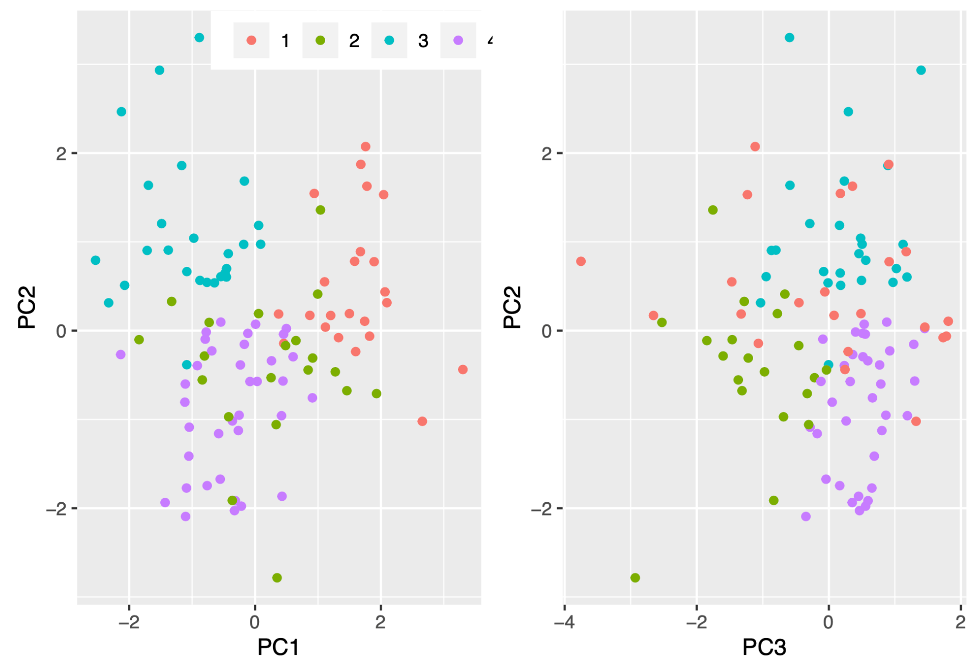
2D plots are kind of like looking at two different sides of a cube, and then the 3D plots offer another perspective. Clusters 3 and 4 (in blue and purple) are well-clustered, while 1 and 2 appear highly variable.

It could be interesting to include clusters we found in the predictive model, but for now I’ll trust that any information we glean from the cluster solution is already included in the raw data. Now, onto the exciting stuff.

IV. Modeling

All statistical learning models were selected and tuned through n-fold cross validation. Here was the algorithm: The model is trained on finalists from all seasons but one. The predicted probabilities of winning for the left-out season finalists are obtained from the trained model, and the person with the highest probability in the final 2 or final 3 is declared the winner.

I considered various models but eventually landed on a neural network with logistic outputs. I ran into issues with nonlinear models like boosted trees and k-nearest neighbors where the model was yielding equal win probabilities and hence predicting multiple winners per season. Neural network predictions did not have the same issue. I used the nnet package to fit the model.

Now, what can we learn from it? We can look at relative feature importance to see which variables have the largest contribution in predictions. I’ll use caret package, which uses Recursive Feature Elimination (RFE) to determine the importance measures.

And we can also use partial dependence plots (I use ALE plots here) to see the isolated effects of each variable.

It is slightly annoying to interpret the variables since the scales are normalized, but we can look at the curve to provide some explanations.

• Age follows a roughly linear trajectory, meaning younger finalists are more likely to win the show.
• majorityvote has a very interesting curve. Win probability is maximized at a little below the average and sharply declines as majorityvote approaches 1. The way I see it is that players who didn’t always vote with the majority are favored, but not to the extent where the percentage is extremely low (if a finalist never knew what was going on and always voted against the crowd, that’s viewed negatively.) But when the percentage is too high, close to 100%, then the finalist is probably viewed by the jury as cunning and devious which also works against the finalist’s favor.
• Number of immunity idols (necklaces) was probably the most surprising here, where fewer idols didn’t have a positive effect (if you see the scale for x_2 (necklaces), main effect at y-axis at the lower end is 0) but more idols hurt the finalists’ chances.
• Appearance didn’t appear to be one of the more important variables, and it is most likely heavily influenced by one particular data point for Season 22 when Rob “Boston Rob” Mariano won Survivor on his 4th try.

V. Bootstrap Estimates

Now that I have my model tuned, I can repeat this a bunch of times! Bootstrapping essentially just means that I shuffled the datapoints to re-fit the model many many times, and aggregating predictions from each model.

For each season, I generated 10000 predictions of who the winner is going to be, with a model trained on a resampling with replacement of the 39 other seasons. That is a whopping 400,000 neural networks fit! Thankfully I was able to set up this code to run on the MSiA servers overnight.

How should we interpret these results? The way I look at it is, since the predictions for each season are done using a model trained on the other 39, a high predicted% indicates that the way the finalist played “a textbook game”. The model says Chris from Vanuatu or Ethan from Africa had a game style possibly similar to those we saw before, and the previous contestants that played like they did usually won.

For Jeremy and Yul, the opposite. They were possibly in the finals with a textbook contestant, and the model saw Jeremy winning only 450 out of 10000 simulations of the season. Against all odds, these winners were able to claim the title in the end.

Another interesting table to look at is the non-winners with the highest predicted%.

The model says these shoo-ins could not convince the jury. Kelly and Colby came to the end with lots of immunity idols won along the way, but they lost. For Spencer and Woo, it is hard to tell. Woo was likely favored due to the fact that he was in the majority vote most of the time, and Spencer was relatively young at 23 when he played in Season 31: Cambodia – Second Chance, a returning player season with most contestants in their 30s and 40s.Table 4.3: Highest (false) prediction rates for finalists who did not win

Conclusions

This exercise was less about building the best predictive model to help me hit the jackpot at bets.com for season 41, and more about coming to understand various intricacies of gameplay and strategy within the realm of my favorite TV show. Normally, I don’t care much to interpret what a statistical model predicts a historical datapoint, but in the case of this particular dataset, one datapoint is a 13-episode season with story arcs, big personalities and iconic challenges, so reviewing the output of my n-fold cross validation was actually enjoyable for once. I feel like I gained some understanding as to what some past winners had to set them apart from the rest, and how each of these winners fit in (and not fit in) with each other.

How well did I do in the two questions I set out to answer? Since there were no previous analysis efforts (as far as I could search on the Internet), feature engineering & selection was difficult. But I think just by trial-and-error in things like choosing an appropriate distance measure metric to see finalist voting history similarity to the jury taught me a lot about data integrity and dangers of boiling an entire season’s worth of effort to a number. As far as trying to understand how each of my variables come in to play, I was not entirely thrilled with a rather low correct classification rate of my model, but it gave me some interesting insight on how age and immunity idols in particular affect finalists’ chances of winning.

Two big missing variables for me here are race and gender. In my personal opinion, demographics undoubtedly play a huge role in the personal relationships that the castaways form, just like in real life. I would love to repeat the analysis in the future with some demographic data as well to see if it improves the correct classification rate at all.

In any case, you can find me watching Survivor in my Engelhart apartment until I finish all 40 seasons.

References

Bertelsen, B. (2013, December 9). Validity Index Pseudo F for K-Means Clustering. Cross Validated. https://stats.stackexchange.com/questions/79097/validity-index-pseudo-f-for-k-means-clustering.

Brownlee, J. (2019, August 8). A Gentle Introduction to the Bootstrap Method. Machine Learning Mastery. https://machinelearningmastery.com/a-gentle-introduction-to-the-bootstrap-method/.

CBS. (2020, February 5). Survivor (Official Site). https://www.cbs.com/shows/survivor/.

Garbade, D. M. J. (2018, September 12). Understanding K-means Clustering in Machine Learning. Medium. https://towardsdatascience.com/understanding-k-means-clustering-in-machine-learning-6a6e67336aa1.

scikit-learn. (n.d.). Feature selection – RFE. https://scikit-learn.org/stable/modules/feature_selection.html#rfe.

Singh, A. (2019, September 15). Dimensionality reduction and visualization using PCA(Principal Component Analysis). Medium. https://medium.com/@ashwin8april/dimensionality-reduction-and-visualization-using-pca-principal-component-analysis-8489b46c2ae0.