A great deal of psychological analysis is dependent on the results of statistical testing. However, some of the graphs we get from stats can be messy and hard to work with. Histograms, for example, are not great for determining the shape of a distribution, because the they are heavily reliant on the number of “bins” used.

For example, if we were to look at the age distribution of people in the United States, we could use a histogram to show the percentage of people in each age group, and it would look a little like this:

It is pretty hard to look at this graph and see how ages are distributed within each bin. For example, how is one to know how much of the population is 12 years old if that age group is encompassed in a bin of 10 to 20 year-olds? In Calculus, there are a few ways to interpret and transform those pesky histograms into curves we can easily work with, that are more representative of all the data.

Density Functions

The density function formula is useful when one wants to smooth out a histogram with a curve where the area below it is equal to 100% of the data. This curve shows the the way in which numerical observations are distributed through a population, and summarizes the percentages across a histogram by consolidating all of the information under the curve. The curve is defined by the integral between the lowest and highest possible points, and the formula to find it is:

$\int _b ^a p(x)dx$

Once computed, the curve looks as follows, making it easier to interpret the probability that the age of a randomly selected person in a sample would fall into each range of ages.

* Because age is a continuous variable, we cannot compute the possibility of a person being any specific age, but we can see how the data is distributed between age groups in a more coherent way than a histogram can show us.

Cumulative Distribution Functions

Another way to characterize distributions is by using the cumulative distribution function. This function essentially gives the same data that the density function gives, but it offers the area under the curve from minus infinity to whatever x value you want.

This formula is as follows:

$\int _{ -\infty} ^t p(x)dx$ = the fraction of the population having values of x below t

 

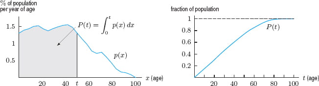
For example, if you want to find the percent of people under the age of 50, you would add the areas of each box below the 50-year mark, leaving you with $P(x) = 0.73$, or $73\%$ of the population between the ages of 0-50.

Normal Distributions

We rely mostly on normal distributions in psychological testing. These normal curves are bell-shaped, and represent the probability that a randomly chosen person from a population will fall within a certain range of data points from the mean.

To calculate the area under the curve in these ranges, we must first find a number that represents a set distance from the mean (which is the highest point of the curve). This number is called the standard deviation, which is found with the following formula:

$\sigma = \sqrt \frac {\sum x – \bar x}  {n}$

The empirical rule states the 68% of the data will fall within +/- 1 standard deviation of the mean, 95% of data will fall within +/- 2 standard deviations of the mean, and 99.7% of data will fall within +/- 3 standard deviations  of the mean. This is defined by integration as well, through the use of the following density function formula:

$ \int_{b}^{a} = \frac {1} {\sigma \sqrt 2 \pi} e^{-(x- \mu)^2  / (2 \sigma ^2)}dx$

($\mu$ is the mean and $\sigma$ is the standard deviation in this equation)

This formula is most useful when the standard deviation is equal to 1, otherwise you would need to also compute a z-score, but this post is already more than 600 words so we won’t get into that :).

This formula simply confirms the empirical rule, where if you were to plug in the mean and a standard deviation of 1, and attempted to find the area under the curve that fell in the ranges mentioned above, you would compute the same percentages. However, in order to compute this for a standard deviation that is not equal to 1, you would need to compute a z-score and get into a little more detailed statistical analysis.

You can also use probability to find the percentile a specific score falls within the distribution, and the likelihood that a randomly chosen person will have any one specific score. Knowing how to work with normal distributions is really useful, especially if you are in a class where the professor grades on a curve.

 

 

Sources:

Applied Calculus, 5th Edition. John Wiley & Sons
Chapter 7, Probability
https://learning.oreilly.com/library/view/applied-calculus-5th/9781118174920/06_chapter07.html#