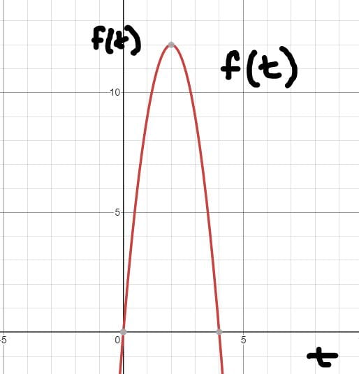
Saitama, also known as One Punch Man, is an extremely powerful human being that can wipe out planets with a single swing of his fist. How he obtained his strength? No one knows. What we are able to know, however, is the maximum height of a rock he tosses (at bare minimum strength, of course) and the time it takes for the rock to reach that height. For instance, say Saitama effortlessly tosses a pebble up into the air, where the height $h$ in kilometers at any time $t$ in seconds is given by the function:

$$h(t) = 5 + 12t – 3t^2$$

Using the power of calculus, we are able to discern that the rock thrown reaches a maximum height of 17 kilometers at the time of 2 seconds. Yeesh.

How did we figure this out? Let’s break it down.

If we graphed out the function, it would look something like this:

As you can see, in the case of a smooth, continuous graph of a function, the maximum height is the highest point, which would lead us to think that the minimum is the lowest point of the graph relative to a point $p$, which it is.

These highest and lowest points are called maxima and minima, and in the case of this blog post we will be focusing on a more condensed spectrum realtive to point $p$, so we will refer to them as local maxima and minima. They are collectively called local extrema.

Looking at a graph, the local maxima and minima are the points where the graph flattens out and changes from increasing to decreasing, or vice versa. When the graph is flat, that means the slope is zero. We can find out when the slope is zero using the derivative.

(Image source: Just Contemplating a Few Things. Digital Image. Gfycat.com)

Derivatives 

The first concept we ought to have in our arsenal in order to figure out things like what the maximum height of a rock thrown by Saitama (at bare minimum power) is, is the derivative. Fundamental to calculus, the derivative is essentially figuring out the slope of a function. Put in other words, the derivative tells us the rate at which something occurs at a given point. Looking at the previous function

$$h(t) = 5 + 12t – 3t^2$$

we derive the derivative using a number of rules.

Just a refresher, the first rule we use is the constant rule, which says that the slope of any constant $c$ is 0. So the 5 in the above function is nullified.

The second rule we utilize is that the slope of a line $ax$ has a derivative of $a$. In the example, $12t$ is converted into merely $12$ as the derivative.

Finally, the power rule, which says that any function $x^n$ has a derivative of $nx^{n-1}$. In the above case, $3t^2$ becomes $6t$ because $3\times 2= 6$ and $2-1 = 1$.

The same rules are applied to the Derivative to find the Second Derivative, which can be thought of as the rate of change of the rate of change (woah).

Now that we know how to find both the derivative and second derivative, there’s so much we can calculate.  We can find, for instance, where the derivative is zero, and thus what the maximum height of Saitama’s tossed pebble is.

Looking at our function:

$$h(t) = 5 + 12t – 3t^2$$

we find the derivative using the previously mentioned rules:

$$h'(t) = 12 – 6t$$

then we set the derivative equal to $0$ in order to find the value of $t$, the time when the slope is $0$.

$$0 = 12 – 6t$$

$$-12 = -6t$$

$$\frac{-12}{-6} = \frac{-6t}{-6}$$

$$2 = t$$

Once the time that the rock reaches its maximum height is known, we can calculate the maximum height by substituting the value of $t$ we have into the original equation.

$$h(2) = 5 + 12(2) – 3(2)^2$$

$$h(2) = 5 + 24 – 12$$

$$h(2) = 17 km/sec$$

That’s how we can derive a local maxima if we are given a function. Now let’s delve deeper into this concept by looking at graphs and their relationship with the first and second derivative.

We know that

if $f'(x) > 0$ on an interval, then $f(x)$ is increasing on that interval.

if $f'(x) < 0$ on an interval, then $f(x)$ is decreasing on that interval.

if $f”(x) > 0$ on an interval, then $f(x)$  is concave up on that interval.

if $f”(x) < 0$ on an interval, then $f(x)$ is concave down on that interval.

Knowing this, we can do something called the Second Derivative Test to discern whether or not the graph of a function has a local maxima or minima.

When a function’s derivative is $0$ at point $p$, then we can determine if it is a local maximum or minimum depending on whether or not the second derivative is less than, greater than, or equal to $0$. According to the principles mentioned above, if it is less than, the graph is concave down and the point is a local maximum. If it is greater than, the graph is concave up and the point is a local minimum. For instance, let’s look at a function with the derivative $f(t) = 12 – 9t$ which is a negative slope.

The second derivative would be $-9$ , which is less than $0$ which would mean that the original function is concave down and that there is a local maximum, which looking at the graph, appears to be true

The First Derivative Test can also be used, which says that if $f'(t)$ goes from positive to negative after passing the point where the slope is $0$, then it is a local maximum. The reverse holds true for local minima.

The point where the slope, or $f'(t)$ is equal to $0$ or is undefined is known as a critical point, which makes it true that all maxima and minima are critical points. However, not all critical points are maxima or minima, which can be seen from the following examples of graphs.

$f(x) = x^3 + 2$

Though there is a critical point because there is a point where the slope is $0$, there is neither a minimum or maximum because the slope does not change from positive to negative or negative to positive.

Keeping all of these rules in mind, we are able to discern when and at what height Saitama’s thrown pebble reaches its maximum height.

(image source: Saitama. Digital Image. Konbini.com)

Sources

Applied Calculus, 5th Edition. John Wiley & Sons
Chapter 4, Using the Derivative
https://learning.oreilly.com/library/view/applied-calculus-5th/9781118174920/06_chapter07.html#

Desmos Graphing Calculator. (2015). Desmos Graphing Calculator. [online] Available at: https://www.desmos.com/calculator?create_account