Antiderivatives and The Fundamental Theorem of Calculus

Antiderivatives and the Fundamental Theorem of Calculus

Antiderivatives

Before we can understand what an anti-derivative is, we must know what a derivative is. So, let’s recap: a derivative is the amount by which a function is changing at one given point. In other words, the derivative is defined as the “instantaneous rate of change.” For example, if we were looking at the a problem about how fast a plane is traveling at $(t)$ hours, we would need to find the derivative at time $(t)$ hours in order to find that rate of change in that particular time. Therefore, the speed is the derivative of distance with respect to time—so if the plane is y miles from where it departed at time $(t)$ hours, then its speed is  $\frac{dy}{dt}$  miles per hour.

Now that we know what a derivative is, we can talk about antiderivative. An antiderivative is just as obvious as the name sounds: it is a function that is the reverse of the derivative. (I like to think of it as what the equation is before it becomes differentiated). In calculus terms (and according to the textbook), of $F(x)$ is $f(x)$, that is, if $F′(x) = f(x)$, then we call $F(x)$ an antiderivative of $(x)$. For example, if $f’ (x)$ is $x^2$, then the antiderivative- that’s “F”- will be the integral of that function which is written as (write integral sign x^2 dx) which is equal to $\frac{1}{3x³}+ C$ And remember, while a function only has one derivative, it has infinitely many antiderivatives. But the antiderivatives all differ by a constant, and all of the antiderivatives of $x²$ take the form $\frac{1}{3x³}+ C$ for some constant C.

The Fundamental Theorem of Calculus

As we talked about in lecture, the Fundamental Theorem of Calculus shows the relationship between derivatives and integration and states that if f is the derivative of another function $F$ then, $\int_{a}^{b} f(x)dx$= $F(b)-F(a)$.

Therefore, since  $F$  is the antiderivative of  $f$  to find  $\int_{a}^{b} f(x)dx$  we would find the antiderivative  $F$  and then use that to evaluate $F(b)-F(a)$.

So, using the example provided earlier, let’s evaluate $x^2$ using the fundamental theorem of calculus.

  1. We know that the anti-derivative of $x^2$ is [ $\frac{1}{3x³}+ C$ ]
  2. So, $\int_{a}^{b} f(x^2)dx$ = [ $\frac{1}{3x³}+ C$ ]
  3. [ $\frac{1}{3(a)³}+ C$ ] – [ $\frac{1}{3(b)³}+ C$ ]
  4.  And finally, $\int_{a}^{b} f(x^2)dx$ = [ $\frac{1}{3(a)³}+ C$ ] – [ $\frac{1}{3(b)³}+ C$ ]

Let’s Practice!

In the real world, antiderivatives and the Fundamental Theorem of Calculus are important for lots of things, and it is especially useful for determining how much things grow within an interval of time. We can apply this theorem to a business. Let’s take the popular movie and tv streaming service, Netflix, for example. Netflix started in 1997. If we wanted to determine how much money Netflix has made from 1997 to 2019, we could use the fundamental theorem of calculus to determine this. Netflix is growing at rate of  $1997+15\cdot{x^.30}$

1.  Our upper limit is 22 and our lower limit is 0 (because 2019-2019=22 years and 1997 is the initial year).

2. So, $\int_{0}^{22} f(1997+15\cdot{x^.30})dx$

3. And the antiderivative of $1997+15\cdot{x^.30}$  is [$\frac{150x^\frac{13}{10}}{13} +C$]

4. $\int_{0}^{22} f(1997+15\cdot{x^.30})dx$ = $\left[\frac{150x^\frac{13}{10}}{13}\right]_{0}^{22} $

5. [$\frac{150(22)^\frac{13}{10}}{13}$] – [$\frac{150(0)^\frac{13}{10}}{13}$]

6. So, our answer is that Netflix made a total $44575.64880801436 between the years of 1997 and 2019.

In conclusion…

Antiderivatives and the Fundamental Theorem of Calculus are useful for finding the total of things, and how much things grew between a certain amount of time.


DISCLAIMER-

The numbers used in the Netflix example are completely fictional and were made up for the purposes of the example (except for the fact that is was founded in 1997 which is completely factual).

Probability

A great deal of psychological analysis is dependent on the results of statistical testing. However, some of the graphs we get from stats can be messy and hard to work with. Histograms, for example, are not great for determining the shape of a distribution, because the they are heavily reliant on the number of “bins” used.

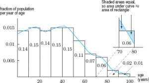
For example, if we were to look at the age distribution of people in the United States, we could use a histogram to show the percentage of people in each age group, and it would look a little like this:

It is pretty hard to look at this graph and see how ages are distributed within each bin. For example, how is one to know how much of the population is 12 years old if that age group is encompassed in a bin of 10 to 20 year-olds? In Calculus, there are a few ways to interpret and transform those pesky histograms into curves we can easily work with, that are more representative of all the data.

Density Functions

The density function formula is useful when one wants to smooth out a histogram with a curve where the area below it is equal to 100% of the data. This curve shows the the way in which numerical observations are distributed through a population, and summarizes the percentages across a histogram by consolidating all of the information under the curve. The curve is defined by the integral between the lowest and highest possible points, and the formula to find it is:

$\int _b ^a p(x)dx$

Once computed, the curve looks as follows, making it easier to interpret the probability that the age of a randomly selected person in a sample would fall into each range of ages.

* Because age is a continuous variable, we cannot compute the possibility of a person being any specific age, but we can see how the data is distributed between age groups in a more coherent way than a histogram can show us.

Cumulative Distribution Functions

Another way to characterize distributions is by using the cumulative distribution function. This function essentially gives the same data that the density function gives, but it offers the area under the curve from minus infinity to whatever x value you want.

This formula is as follows:

$\int _{ -\infty} ^t p(x)dx$ = the fraction of the population having values of x below t


For example, if you want to find the percent of people under the age of 50, you would add the areas of each box below the 50-year mark, leaving you with $P(x) = 0.73$, or $73\%$ of the population between the ages of 0-50.

Normal Distributions

We rely mostly on normal distributions in psychological testing. These normal curves are bell-shaped, and represent the probability that a randomly chosen person from a population will fall within a certain range of data points from the mean.

To calculate the area under the curve in these ranges, we must first find a number that represents a set distance from the mean (which is the highest point of the curve). This number is called the standard deviation, which is found with the following formula:

$\sigma = \sqrt \frac {\sum x – \bar x}  {n}$

The empirical rule states the 68% of the data will fall within +/- 1 standard deviation of the mean, 95% of data will fall within +/- 2 standard deviations of the mean, and 99.7% of data will fall within +/- 3 standard deviations  of the mean. This is defined by integration as well, through the use of the following density function formula:

$ \int_{b}^{a} = \frac {1} {\sigma \sqrt 2 \pi} e^{-(x- \mu)^2  / (2 \sigma ^2)}dx$

($\mu$ is the mean and $\sigma$ is the standard deviation in this equation)

This formula is most useful when the standard deviation is equal to 1, otherwise you would need to also compute a z-score, but this post is already more than 600 words so we won’t get into that :).

This formula simply confirms the empirical rule, where if you were to plug in the mean and a standard deviation of 1, and attempted to find the area under the curve that fell in the ranges mentioned above, you would compute the same percentages. However, in order to compute this for a standard deviation that is not equal to 1, you would need to compute a z-score and get into a little more detailed statistical analysis.

You can also use probability to find the percentile a specific score falls within the distribution, and the likelihood that a randomly chosen person will have any one specific score. Knowing how to work with normal distributions is really useful, especially if you are in a class where the professor grades on a curve.


Sources:

Applied Calculus, 5th Edition. John Wiley & Sons
Chapter 7, Probability
https://learning.oreilly.com/library/view/applied-calculus-5th/9781118174920/06_chapter07.html#


Local Extrema

Saitama, also known as One Punch Man, is an extremely powerful human being that can wipe out planets with a single swing of his fist. How he obtained his strength? No one knows. What we are able to know, however, is the maximum height of a rock he tosses (at bare minimum strength, of course) and the time it takes for the rock to reach that height. For instance, say Saitama effortlessly tosses a pebble up into the air, where the height $h$ in kilometers at any time $t$ in seconds is given by the function:

$$h(t) = 5 + 12t – 3t^2$$

Using the power of calculus, we are able to discern that the rock thrown reaches a maximum height of 17 kilometers at the time of 2 seconds. Yeesh.

How did we figure this out? Let’s break it down.

If we graphed out the function, it would look something like this:

As you can see, in the case of a smooth, continuous graph of a function, the maximum height is the highest point, which would lead us to think that the minimum is the lowest point of the graph relative to a point $p$, which it is.

These highest and lowest points are called maxima and minima, and in the case of this blog post we will be focusing on a more condensed spectrum realtive to point $p$, so we will refer to them as local maxima and minima. They are collectively called local extrema.

Looking at a graph, the local maxima and minima are the points where the graph flattens out and changes from increasing to decreasing, or vice versa. When the graph is flat, that means the slope is zero. We can find out when the slope is zero using the derivative.

(Image source: Just Contemplating a Few Things. Digital Image. Gfycat.com)

Derivatives 

The first concept we ought to have in our arsenal in order to figure out things like what the maximum height of a rock thrown by Saitama (at bare minimum power) is, is the derivative. Fundamental to calculus, the derivative is essentially figuring out the slope of a function. Put in other words, the derivative tells us the rate at which something occurs at a given point. Looking at the previous function

$$h(t) = 5 + 12t – 3t^2$$

we derive the derivative using a number of rules.

Just a refresher, the first rule we use is the constant rule, which says that the slope of any constant $c$ is 0. So the 5 in the above function is nullified.

The second rule we utilize is that the slope of a line $ax$ has a derivative of $a$. In the example, $12t$ is converted into merely $12$ as the derivative.

Finally, the power rule, which says that any function $x^n$ has a derivative of $nx^{n-1}$. In the above case, $3t^2$ becomes $6t$ because $3\times 2= 6$ and $2-1 = 1$.

The same rules are applied to the Derivative to find the Second Derivative, which can be thought of as the rate of change of the rate of change (woah).

Now that we know how to find both the derivative and second derivative, there’s so much we can calculate.  We can find, for instance, where the derivative is zero, and thus what the maximum height of Saitama’s tossed pebble is.

Looking at our function:

$$h(t) = 5 + 12t – 3t^2$$

we find the derivative using the previously mentioned rules:

$$h'(t) = 12 – 6t$$

then we set the derivative equal to $0$ in order to find the value of $t$, the time when the slope is $0$.

$$0 = 12 – 6t$$

$$-12 = -6t$$

$$\frac{-12}{-6} = \frac{-6t}{-6}$$

$$2 = t$$

Once the time that the rock reaches its maximum height is known, we can calculate the maximum height by substituting the value of $t$ we have into the original equation.

$$h(2) = 5 + 12(2) – 3(2)^2$$

$$h(2) = 5 + 24 – 12$$

$$h(2) = 17 km/sec$$

That’s how we can derive a local maxima if we are given a function. Now let’s delve deeper into this concept by looking at graphs and their relationship with the first and second derivative.

We know that

if $f'(x) > 0$ on an interval, then $f(x)$ is increasing on that interval.

if $f'(x) < 0$ on an interval, then $f(x)$ is decreasing on that interval.

if $f”(x) > 0$ on an interval, then $f(x)$  is concave up on that interval.

if $f”(x) < 0$ on an interval, then $f(x)$ is concave down on that interval.

Knowing this, we can do something called the Second Derivative Test to discern whether or not the graph of a function has a local maxima or minima.

When a function’s derivative is $0$ at point $p$, then we can determine if it is a local maximum or minimum depending on whether or not the second derivative is less than, greater than, or equal to $0$. According to the principles mentioned above, if it is less than, the graph is concave down and the point is a local maximum. If it is greater than, the graph is concave up and the point is a local minimum. For instance, let’s look at a function with the derivative $f(t) = 12 – 9t$ which is a negative slope.

The second derivative would be $-9$ , which is less than $0$ which would mean that the original function is concave down and that there is a local maximum, which looking at the graph, appears to be true

The First Derivative Test can also be used, which says that if $f'(t)$ goes from positive to negative after passing the point where the slope is $0$, then it is a local maximum. The reverse holds true for local minima.

The point where the slope, or $f'(t)$ is equal to $0$ or is undefined is known as a critical point, which makes it true that all maxima and minima are critical points. However, not all critical points are maxima or minima, which can be seen from the following examples of graphs.

$f(x) = x^3 + 2$

Though there is a critical point because there is a point where the slope is $0$, there is neither a minimum or maximum because the slope does not change from positive to negative or negative to positive.

Keeping all of these rules in mind, we are able to discern when and at what height Saitama’s thrown pebble reaches its maximum height.

(image source: Saitama. Digital Image. Konbini.com)

Sources

Applied Calculus, 5th Edition. John Wiley & Sons
Chapter 4, Using the Derivative
https://learning.oreilly.com/library/view/applied-calculus-5th/9781118174920/06_chapter07.html#

Desmos Graphing Calculator. (2015). Desmos Graphing Calculator. [online] Available at: https://www.desmos.com/calculator?create_account


Calculus In Physics Engines

What are Physics Engines?

Physics engines are programs that are used to simulate physical phenomena. These programs have been used for decades by the military, meteorologists, and even video game developers. Their applications range from determining where artillery shells would land, based on several parameters, to simulating a similar situation in a match of Call of Duty or Battlefield. Video games offer a great chance to see how simulations are run. Of course, physics simulations in video games are not solely limited to militaristic phenomena. In fact, the other applications are mostly artful in nature and can lead to downright breathtaking moments for consumers.

What does this have to do with Calculus?

The different applications for physics engines are as interesting as they are extensive, but what does this have to do with calculus and this course in general? As it happens, functions are an integral part of physics engines and programming. Initially the calculus of physics engines in video games was delegated to detecting collisions between in-game objects (such as player characters, rocks, and dust particles) and enacting appropriate responses. However, over the last few decades the engines have been updated to adopt more advanced calculus to the effect of more believable interactions between in-game objects. In order to apply the level of calculus necessary to achieve such effects, physics engines use a segment of code called an integrator. The integrator of a physics engine would take in information of an object at time t and apply that information to formulas in order to determine the new position/vector of said object.

Basic Integrator Formulas and other Determinants

Here are just some of the formulas used by a physics engine integrator:

Position

Derivative: $\mathit{r(t)}$

Integral: $\mathit{r(t)}$ = $r_0 + \int_0^t vdt’$

Velocity

Derivative: $\mathit{v(t)}$ = $\frac{dr}{dt}$

Integral: $\mathit{v(t)}$ = $v_0 + \int_0^t adt’$

Acceleration

Derivative: $\mathit{a(t)}$ = $\frac{dv}{dt} = \frac{d^2r}{dt^2}$

Integral: $\mathit{a(t)}$

This means that the Velocity of an object can be found with the anti derivative of its Acceleration and its Position with the anti derivative of its velocity. It also means that the area determined by the integral of the Acceleration is the total change in velocity, and the area determined by the integral of the Velocity is the displacement of the object. All of which are important for predicting the position of any object from the time a simulation starts to when it ends.

Aside from these important formulas that determine the position/vector of in-game objects, the objects are also subjected to the same laws of physics that we experience in reality. These laws include Isaac Newton’s laws of motion and universal law of gravity, and D’Alembert’s principle which sums all the vectors of an object into one whole vector.

ex. The total work done by a constant Force ($\mathit{F}$) whilst moving an object a distance($\mathit{d}$) is represented by the integral:

$\mathit{W}$ = $\int_a^b F(x)dx$

Although the simulations are not always perfect, the combination of all these factors working together within a physics engine provide an experience that is becoming more realistic every year to the point of being almost indistinguishable from physical phenomena we may see in everyday life. Calculus ultimately plays an important part in how such an engine interprets data from a simulation and returns an appropriate response. It can even be said that without calculus it would be impossible to predict the outcome of a physical phenomenon in a simulation or even in reality.

Sources

Applied Calculus 5th Edition (Hughes-Hallet, Gleason, Lock, Faith, et al.) : 5.1, 5.2

https://faculty.atu.edu/mfinan/2924/cal76.pdf

http://www.ugrad.math.ubc.ca/coursedoc/math103/site2012/keshet.notes/Chapter4.pdf

https://prezi.com/qicki_zqvo9v/the-calculus-of-video-games/


Price Elasticity of Demand

What is price elasticity of demand?

Elasticity of demand is a measure used in economics to determine the sensitivity of demand of a product to price changes. In theory, this measurement can work on a wide range of products, from low priced items like pencils to more significant purchases like cars. Because of this diversity of products, elasticity of demand looks at percent changes in price rather than absolute changes; for example, a \$10 increase for a pack of pencils would be outrageous, while a \$10 increase for a new car would likely go unnoticed. Ultimately, the equation used to determine elasticity of demand can be simply thought of as: how do a price increase of X% affect the demand of product Y? A higher demand elasticity means that consumers are more responsive to changes in the price of the product.

How to determine elasticity of demand

Given that elasticity of demand calculates the relationship between change in price and change in demand, we can begin to derive the formula:

|$\frac{\text{Percent  change  in  demand}}{\text{Percent  change  in  price}}| = |\frac{∆q/q}{∆p/p}$|

This can be further simplified as:

|$\frac{∆q}{q} \cdot \frac{p}{∆p}| = |\frac{p}{q} \cdot \frac{∆q}{∆p}$|

In the above equation ∆p refers to change in price, while ∆q represents the corresponding change in the quantity of the product demanded. Absolute values are used when determining the coefficient of elasticity, because the correlation between price increase and quantity demand can be assumed to always be negative.

For small changes in price, $\frac{∆q}{∆p}$ can be approximated by the derivative $\frac{dq}{dp}$. This means that we can determine elasticity of demand, E, by substituting in the derivatives of ∆q and ∆p into the above formula.

Therefore, E = |$\frac{p}{q} \cdot \frac{dq}{dp}$|

Important values for elasticity of demand

The word “coefficient” is used to describe the values for price elasticity of demand (E). Different coefficient values have various implications for the price elasticity of demand of products:

  • E = 0: demand is perfectly inelastic, meaning that demand does not change at all when the price changes.
  • 0 < E < 1: in these cases, the % change in demand from is smaller than the percentage change in price, and the demand is inelastic.
  • E = 1: here, the % change in demand is exactly the same as the % change in price, which means that the demand is unit elastic. For example, a price increase of %10 would lead to a 10% decrease in demand.
  • E > 1: demand responds more than proportionately to a price increase, so the demand is elastic. For example if a 15% increase in the price of a product corresponds to a 45% drop in demand. In this specific case, E = 3.

The more the demand for a product decreases in relation to the change in price, the more elastic that good is considered.

Application

The demand curve for a product is given by $q = 2000−4p^2$, where p = price. What is the elasticity of the product when the price is \$10?

To solve this problem, first find $\frac{dq}{dp}$. Using the power rule, we know that $\frac{dq}{dp} = -8p$.

We plug this, as well as the price, into the equation, yielding:

$E = |\frac{10}{q} \cdot (-8)$|

To find q, we go back to our original equation.

$q = 2000−4p^2 = 2000−4(10)^2 = 1,600$

Now we have all of the components needed to calculate the price elasticity of demand at price = /$10.

$E = |\frac{10}{400} \cdot (-8)| = .2$

Considering the values of E described above, we know that the product is inelastic at p=10. Another way to think of this is that a 1% increase in price will correspond with an approximately .2% decrease in quantity demand.

Sources:

Applied Calculus 5th Edition (Hughes-Hallet, Gleason, Lock, Faith, et al.) – section 4.6

https://www.tutor2u.net/economics/reference/price-elasticity-of-demand

https://www.extension.iastate.edu/AGDM/wholefarm/pdf/c5-207.pdf

https://www.intelligenteconomist.com/price-elasticity-of-demand/

The Chain Rule

What is the Chain Rule?

The Chain Rule is a mathematical method to differentiate a composition of functions. From this composition of functions, we can discern the functions’ derivatives and their relationships. 

Composition of Functions

A composition of functions is when one variable depends on another variable, which itself depends on another variable. Below are different ways to express this composition of functions. 

  • If y = f(x) and z = g(y), then z depends on y, and y depends on x.
  • This relationship can also be represented in fractional form.
      • $\dfrac{\text{change in } z}{\text{change in } x}$ = $\dfrac{\text{change in } z}{\text{change in } y}$ $\times$ $\dfrac{\text{change in } y}{\text{change in } x}$
  • In addition, Leibniz Notation more succinctly describes this equation.
      • Leibniz Notation: $\dfrac{dz}{dx}$ = $\dfrac{dz}{dy}$ $\times$ $\dfrac{dy}{dx}$

The Chain Rule Formula

  • The Chain Rule formula is $\dfrac{d}{dx}$ [f(g(x))] = f'(g(x)) $\times$ g'(x)
      • In other words, the derivative of the composite function = derivative of the outside function $\times$ derivative of the inside function

Practice with the Chain Rule Formula

The Chain Rule can be used to differentiate many types of functions. Here I have listed 4 practice problems. In all 4 problems, we use the same basic formula, although we find the individual derivatives in different ways.

  • 2 Basic Functions – Use the Chain Rule to differentiate ($x^{3} +2)^{5}$
      • First, assign a term to the outside f(x) and inside g(x) functions
          • KEY: a helpful step to decide which function is which is boxing the inner function
          • outside function f(x) = $x^{5}$
          • inside function g(x) = $x^{3}+2$, with a box around it
      • Plug in the f(x) and g(x) into the Chain Rule formula
          • $\frac{d}{dx}$[f(g(x))] = f'(g(x)) $\times$ g'(x)
          • $5(x^{3} +2)^{4}$ $\times$ $3x^{2}$
  • The Number e – Use the Chain Rule to differentiate y = $e^{x^3+1}$
      • Assign terms
          • outside function f(x) = $e^{x}$
          • inside function g(x) = $x^{3}+1$, with a box around it
      • Plug into formula
          • $\frac{d}{dx}$[f(g(x))] = f'(g(x)) $\times$ g'(x)
          • $e^{x^3+1}$ $\times$ $3x^{2}$
  • Trig Functions – Use the Chain Rule to differentiate f(x) = $e^{6\sin(4x)}$
      • Assign terms
          • outside function f(x) = $e^{x}$
          • inside function g(x) = ${6\sin(4x)}$, with a box around it
      • Plug into formula
          • $\frac{d}{dx}$[f(g(x))] = f'(g(x)) $\times$ g'(x)
          • KEY: the derivative of ${\sin(x)}$ =  ${\cos(x)}$, ${\cos(x)}$ = ${-\sin(x)}$
          • $e^{6\sin(4x)}$ $\times$ 24${\cos(4x)}$
  • Natural Log (ln) – Use the Chain Rule to differentiate $ln(3p^{2}-5)$
      • Assign terms
          • outside function f(x) = ln(x)
          • inside function g(x) = $3p^{2}-5$, with a box around it
      • Plug into formula
          • $\frac{d}{dx}$[f(g(x))] = f'(g(x)) $\times$ g'(x)
          • KEY: the derivative of ln(x) = 1/x
          • $\frac{1}{3p^{2}-5}$ $\times$ 6p

Evaluating Graphs with the Chain Rule

Evaluating graphs involves a different set of skills. The derivative of a function is the slope of the tangent line. In these problems, we must locate the point, and then measure the slope of its tangent line. From there, we can apply the Chain Rule.

Let f and g be functions. Let y=f(x) and z=g(y)

y=f(x) function

z=g(y) function

\

 Find $\frac{dz}{dx}$ when x = 1

In order to find this answer, we will be using the equation $\dfrac{dz}{dx}$ = $\dfrac{dz}{dy}$ $\times$ $\dfrac{dy}{dx}$

    • locate the y value when x=1 on y=f(x) function
        • here it would be y=2
        • y=2 will be helpful for locating the other function’s coordinate
    • find the slope of $\dfrac{dy}{dx}$
        • m = -2
    • using y=2, find the y value at x=2 on z=g(y) function
        • y=2 again
    • find the slope of $\dfrac{dz}{dy}$
        • m = 1
    • multiply these slopes together
        • $\dfrac{dz}{dx}$ =  $\dfrac{dz}{dy}$ $\times$ $\dfrac{dy}{dx}$
        • -2 $\times$ 1 = -2

Evaluating Functions with Their Derivatives

This section is easier than the previous graphing section. We are given the functions and their derivatives. Now, we just plug in!

Let h(x) = f(g(x)) and k(x) = g(f(x))

f(2)=3    f'(0)=0    f'(2)=1   g(2)=0    g'(2) = 3    g'(3) = -2

Evaluate h'(2)

  • Chain Rule Formula: $\dfrac{d}{dx}$ [f(g(x))] = f'(g(x)) $\times$ g'(x)
  • Equivalently, h'(x) = f'(g(x)) $\times$ g'(x) here
      • h'(2) = f'(g(2)) $\times$ g'(2)
      • h'(2) = f'(0) $\times$ g'(2)
      • h'(2) = (0) $\times$ (3)
      • h'(2) = 0

Evaluate k'(2)

  • Chain Rule Formula: $\dfrac{d}{dx}$ [f(g(x))] = f'(g(x)) $\times$ g'(x)
  • Equivalently, k'(x) = g‘(f(x)) $\times$ f'(x) here
      • k'(2) = g'(f(2)) $\times$ f'(2)
      • k'(2) = g'(3) $\times$ f'(2)
      • k'(2) = (-2) $\times$ (1)
      • k'(2) = -2

Real World Applications of the Chain Rule

The Chain Rule can also help us deduce rates of change in the real world. From the Chain Rule, we can see how variables like time, speed, distance, volume, and weight are interrelated.

A horse is carrying a carriage on a dirt path. The amount of ${\text(energy)}$ E (in calories) expended by the horse depends on the ${\text(distance)}$ m (in miles) the horse walks. Also, the distance walked by the horse depends on ${\text(time)}$ t (in hours). If the horse expends 40 calories per mile and the horse walks at a speed of 8 mph, at what rate is the horse expending energy?

  • Chain Rule Formula: $\dfrac{dz}{dx}$ = $\dfrac{dz}{dy}$ $\times$ $\dfrac{dy}{dx}$
  • —————————————————————————————–
  • $\dfrac{dE}{dm}$ = $\dfrac{energy}{time}$
  • —————————————————————————————–
  • $\dfrac{dE}{dm}$ $\times$ $\dfrac{dm}{dt}$
  • —————————————————————————————–
  • $\dfrac{40 calories}{1 mile}$ $\times$ $\dfrac{8 miles}{1 hour}$ = 500 calories
  • —————————————————————————————–
  • The horse expends energy at a rate 500 calories per 1 hour of walking.


Marginal Cost

The Big Idea: Marginal Cost- Derivatives in Economics

In economics, derivatives are applied when determining the quantity of the good or service that a company should produce.

For example: You can model cost as a function of quantity:   $C(x)=(.000001x^3)-(.003x^2)+5x+1000$

You can take the first derivative of this equation to understand the rate of change in cost for each additional product produced:

$C'(x)=(.000003x^2)-.006x+5$→ This is called the Marginal Cost.

As expected, the marginal cost, is positive for all X values. This makes sense because no matter what the quantity is, producing more will result in higher costs. In other words, more production never costs less.

What is its importance??

While considering the average cost of production is important, it is not as relevant as marginal cost. For instance, if it costs a toothbrush company \$300,000 to make 500,000 toothbrushes, each one costs the company \$0.60. However, this doesn’t tell the company how much each new additional toothbrush is costing them to make. It could be \$0.25, or it could be \$0.75. The average cost doesn’t capture this idea while the marginal cost does. This analysis is crucial if a company needs to reduce its cost, while still trying to make as much money as possible.

The marginal cost does increase and decrease. For instance, C'(6) > C'(500), illustrating that when producing 6 units, the cost of the next additional unit is higher than if you were to produce 500 units and wanted to produce the 501st.

$C'(6)=(.000003(6)^2)-.006(6)+5=4.85$

$C'(500)=(.000003(500)^2)-.006(500)+5=2.75$

This concept is called economies of scale; in this case, economies of production. When you are producing more, producing an additional unit is cheaper than when you are producing less.  However, this pattern doesn’t continue forever, since C’ increases and decreases there is a point where it has a minimum. In other words, there is a certain level of production (x) at which the cost of producing one additional product is as low as possible. In the example above, this happens when

$C”(x)=0.$

$C”(x)= .000006x-.006$

$0= .000006x-.006$

$x=1000$

At a production level of 1000 units, the marginal costs is at its minimum. Meaning that producing one additional product costs more than it did previously. This ultimately results in less profit. Given that X= 1000 is an inflection point on the graph of y=c(x), it is concave down for when x> 1000 meaning that the marginal cost is decreasing. The marginal cost is increasing when the function is concave up (x >1000).


Sources:

http://math.hawaii.edu/~mchyba/documents/syllabus/Math499/extracredit.pdf

http://tutorial.math.lamar.edu/Classes/CalcI/BusinessApps.aspx

https://www.economicsonline.co.uk/Definitions/Marginal_cost.html

https://www.investopedia.com/terms/m/marginalcostofproduction.asp


Calculus in Medicine

Pharmacokinetics is the study of how drugs (or any other substances that can be consumed) are processed within the body.

Pharmacokinetics can be broken down into five general steps in which a drug takes its course:

  1. Liberation – the drug is released from its pharmaceutical formulation
    • For example, this would be the point in which the outer core of a pain-relieving gel capsule (ie., Advil) disintegrates to release the medicinal components inside.
  2. Absorption – the drug enters the body through blood circulation
    • This would occur when the medicinal components of the gel enter the bloodstream.
  3. Distribution – the drug is dispersed through the body
    • During this point, the pain-relieving gel provides pain relief as it is being  spread through the blood stream by the body.
  4. Metabolism – the drug is processed and broken down by the body
    • During this point, the pain relieving effects begin to wear off slightly.
  5. Excretion– the drug leaves the body
    • The drug no longer provides pain relief and is excreted by the body.

In order for doctors to prescribe the correct dosage of a drug and provide a regimen for treatment (ie., “take 2 capsules twice a day”),  the drug’s concentration over time must be tracked. This prevents under and over-dosing.

The way that a drug’s concentration over time is calculated is using calculus! In fact, a drugs course over time can be calculated using a differential equation.

In applications of differential equations, the functions represent physical quantities, and the derivatives, as we know, represent the rates of change of these qualities. Therefore, a differential equation describes the relationship between these physical quantities and their rates of change.

In order to create a differential equation that describes the physical quantities of a drug in relation to the rate at which they change, let’s consider the following variables:

$d$ – drug dosage in milligrams

$c$ – the concentration of the drug at any time t

$t$  – time in hours since consumption of drug


In addition to the above variables which seem relatively obvious, the equation also requires the use of :

$k_a$– the absorption constant of a drug

$k_e$ – the elimination constant of drug

$v$ – volume of drug in body

$b$ – bioavailability*

*bioavailability is the amount of the drug which has already been absorbed divided by the total amount of drug available


Calculating the rate of absorption:

In order to calculate the rate of absorption, the equation must include the drug dosage, the absorption constant, and the drug’s bioavailability.

Absorption = $(k_a)(d)(b) \times e^{-at}$

Calculating the rate of  elimination:

In order to calculate the rate of  elimination, the equation must include the elimination constant, the volume of drug distributed throughout the body, and the concentration of the drug that is left.

Elimination = $(k_e)(c)(v)$


Formulating a differential equation:

In order to model our concentration over time, the elimination must be subtracted from the absorption in order to calculate the amount of drug that is left in the body at various time points. 

$\dfrac{dc}{dt}$ = $\dfrac{k_a}{k_a-k_e}$ $[(k_a)(d)(b) \times e^{-at}$ $- (k_e)(c)(v)]$

Drug Concentration vs. Time

The graph above represents a solution to the differential equation.

When actual numbers corresponding to a drug are inserted into the above equation, the graph will tend to generally form as a curve that has a steep positive slope during absorption, levels off once peak drug concentration is reached, and a has a negative slope during elimination.

Consider the following variables

$\dfrac{da_g}{dt}$– the amount of drug being absorbed over time

$\dfrac{de_g}{dt}$ — the amount of drug being eliminated over time

Absorption phase:

In the absorption phase, the drug is being absorbed faster than it is being eliminated, causing the drug concentration to increase.

$\dfrac{da_g}{dt}$ > $\dfrac{de_g}{dt}$

Elimination phase:

The drug is no longer being absorbed and the rate of elimination exceeds the rate of absorption.

$\dfrac{da_g}{dt}$ < $\dfrac{de_g}{dt}$

Medical professionals need calculus!

Without drug specialists in the pharmaceutical industry testing drug concentrations over time and modeling them using calculus, we would not have labels on medication that provide instructions for dosage use.

Although the equation for each drug looks unique depending on its properties and the patient’s anatomy, calculus is necessary for medical professionals to have the ability to map the relationship between drug concentration in the body over time.


Sources:

http://pharmacy.unc.edu/files/2015/06/PK-Book-2014.pdf  (pg. 59-62)

https://math.stackexchange.com/pharmacokinetics-differential-equations

https://www.boomer.org/c/p1/Ch08/Ch0802.html

https://www.ausmed.com/cpd/articles/pharmacokinetics-and-pharmacodynamics

Typesetting mathematics

This blog post is a quick introduction to typesetting mathematical notation using LaTeX commands, which in WordPress is done using MathJax.

You can start typing mathematical notation by entering a dollar sign, and then when you’re done enter another dollar sign.

Example: The square of a number is given by $x^2$ (\$x^2\$)

If you actually want to type a dollar sign, put a backslash before it. For example, typing \\\$300 gives: \$300.

Most of the commands for typing mathematics are pretty intuitive:

  • Most stuff: Just type it. For example, $a+b+c$ (\$a+b+c\$)
  • Multiplication: $12 \times 20$ (\times) or $12 \cdot 20$ (\cdot) but not $12*20$ (*)
  • Fractions: $\frac{x^2 + y^2}{a^2 + b^2}$ or $\dfrac{x^2 + y^2}{a^2 + b^2}$ (\frac{top}{bottom} or \dfrac{top}{bottom})
  • Radicals: $\sqrt{100}$ or $\sqrt[5]{100}$ (\sqrt{100} or \sqrt[5]{100})
  • Exponents: $e^-x^2$ is bad (\$e^-x^2\$) but $e^{-x^2}$ is good (\$e^{-x^2}\$)
  • Subscripts: $a_2$ (\$a_2\$) or $x_{100}$ (\$x_{100}\$), but not $x_100$ (\$x_100\$)
  • Trig and log functions: $\sin(x), \cos(x), \ln(x)$ (\sin, \cos, \ln)
  • Parentheses around fractions: $\sin ( \dfrac{\pi}{4} )$ (\$\sin( \dfrac{\pi}{4} )\$) vs $\sin \left( \dfrac{\pi}{4} \right)$ (\$\sin \left( \dfrac{\pi}{4} \right)\$)

Sometimes we want to put long equations on their own line so that they don’t clutter a paragraph. We can do this using \$\$double dollar signs\$\$ on both ends: $$\dfrac{d}{dx} ( x^2 + \sin(x) + e^x) = 2x + \cos(x) + e^x$$

Common mistakes:

  • Forgetting to close a brace or dollar sign: $\sqrt{x^2 + e^x + \ln(2x)$
  • Using (parentheses) instead of {braces} for arguments to commands: $\sqrt(100 + 2x)$ vs $\sqrt{100+2x}$
  • Exponents without braces surrounding them: $e^100$ vs $e^{100}$
  • Misspelling a command

Example putting this together:

$\dfrac{d}{dx} ( \sqrt{1 + x^2} ) = \dfrac{x}{\sqrt{1+x^2}}$

Welcome to Re(calc)ulated!

This is the course blog for Math 211 (Short Course in Calculus) in Spring 2019. As part of the course, students will be writing posts on this blog about anything related to calculus.

Our first student post will be on Monday, May 6th, by Nejla, who will tell us about applications of calculus in medicine.

I’ll make another post soon containing a quick guide for using MathJax to typeset mathematical notation using LaTeX commands.