Simple College Football Rankings System

| By Macon McLean |

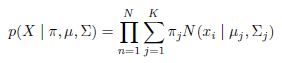
With intense rivalries and unparalleled upsets, college football is a sport like no other.  As an avowed fan, I find each Saturday is more exciting than the last, as the postseason picture becomes clearer with each passing week.  All teams are fighting for bowl games, and for the especially talented schools, a national championship is the ultimate goal.  But not every school can vie for a title:  only the schools ranked in the top four at season’s end can compete in the College Football Playoff.  This simple fact weighs on the minds of coaches, players, and fans every single Saturday.

After the season’s halfway point, while coordinators and coaches spend Mondays discussing game plans and debating tactics, there’s a wider-ranging discussion going on among another group of football geeks:  the College Football Playoff Selection Committee.  Each Tuesday in the second half of the season, the Selection Committee faces the impossible task of ranking the top teams in college football.  This is the sole charge of these arbiters of the gridiron, who number among them former university athletic directors, head ball coaches, and even a Secretary of State (Condoleezza Rice is a voting member).  After each of their weekly meetings, the Committee issues official rankings that determine placement in postseason games, including the vaunted Playoff itself.

Creating these rankings is far from simple.  Given the nature of the sport, establishing a college football hierarchy turns out to be a uniquely challenging problem.  A school’s record often belies its true ability:  an undefeated team from a weaker athletic conference might be propped up by a softer strength of schedule; a squad with two close defeats at the hands of powerhouses (think Michigan and Ohio State) might be better than some teams with fewer losses.  Turnover luck, injuries, and significant variance in scheme all make this feel like a difficult and seemingly arbitrary judgment.  The most significant challenge, however, is independent of on-field performance:  there are 128 teams to evaluate.

Apart from the logistical issues of watching every team in the country, having this many teams makes it hard to compare them directly.  Unlike professional football, top-level college football teams play only a small fraction of their possible opponents.  In the NFL’s regular season, a team will play thirteen of thirty-one candidate opponents; in college football, this number is, at most, fourteen of 127.  This makes it very hard to compare many pairs of teams, as common points of comparison are few and frequently nonexistent.  And due to schools’ membership in athletic conferences, the pool of possible opponents to fill the already small schedule is significantly restricted in size; all ten members of the Big 12 conference, for example, play 75% of their yearly regular season games against each other.

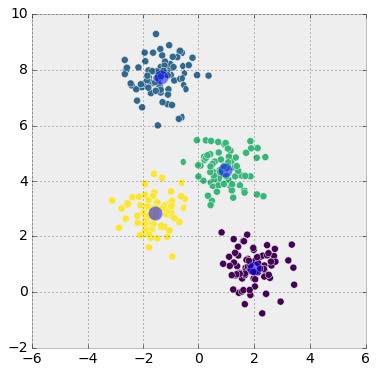
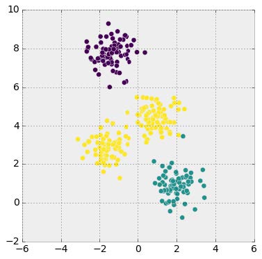
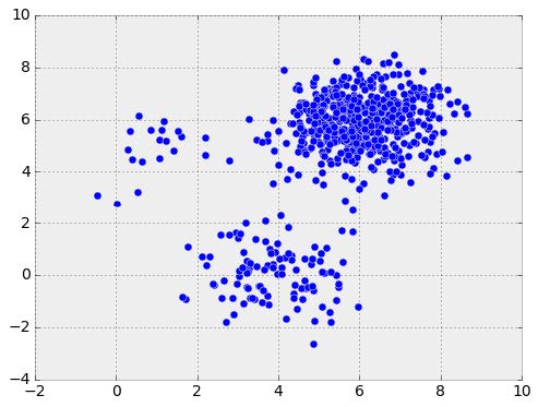
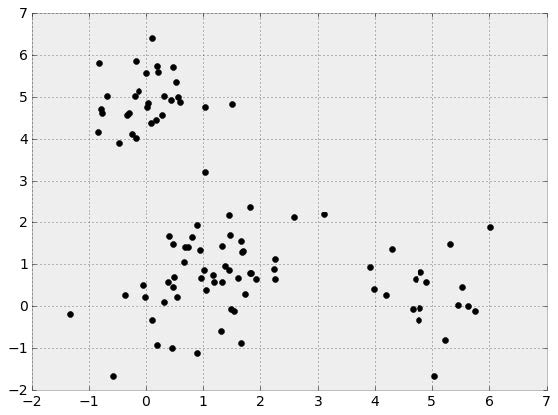
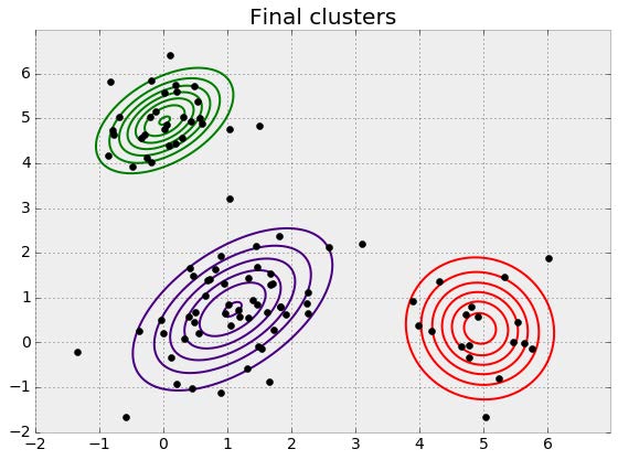
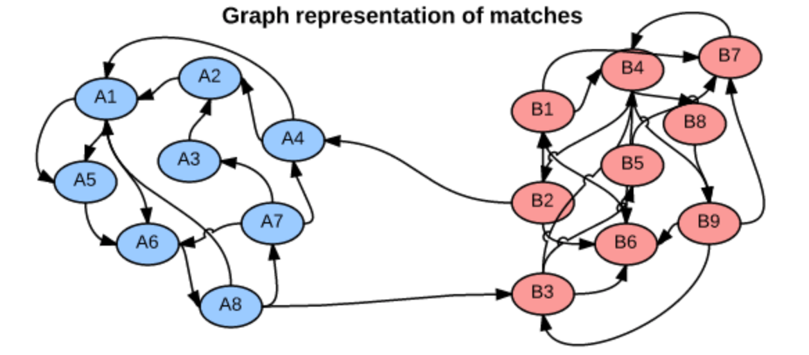
We can think of head-to-head matchups as a way of connecting teams in a graph, a mathematical and visual representation of a network.  Each school is a node and each game serves as an edge connecting two nodes.  College football graphs are often like this picture below, with dense clusters (conferences) each having a few connections to other dense clusters.  This illustrates the problem – the graph is not particularly well-connected, making human application of the transitive property unreliable, and sometimes, impossible.  Eventually all the clusters link up, but it’s not as densely connected as the NFL, and has far fewer data points for comparing teams across conferences.

https://davidabelman.wordpress.com/2015/03/02/modelling-football-team-strength-using-pagerank/

So how does the Selection Committee even approach this problem of comparing teams across conferences?  They base their rankings on the “eye test,” i.e., estimating how talented they believe a squad to be simply by watching them play, independent of any and all advanced metrics.  Though they take into consideration other factors like strength of schedule, head-to-head results, and conference championships, what they see in the “eye test” is the primary evidence.  If this all sounds a bit questionable to you, you’re not alone; the webpage on Selection Committee Protocol begins with “Ranking football teams is an art, not a science.”

Recognizing the difficulty of this task, some enthusiasts have developed more analytically-oriented approaches to ranking teams.  A commonly referenced system is the S&P+ rankings, which use play-level and drive-level data from all college football games to measure four factors:  efficiency, explosiveness, field position, and finishing drives.  However, the Selection Committee is loath to integrate systems like the S&P+ into their proceedings too formally:  the Playoff Committee is the immediate successor to the BCS rankings system, an oft-maligned combination of polls and computer rankings whose inscrutability was, in part, the author of its demise.

So, how could the Selection Committee rank teams in a way that is simple, connected, and not overly dependent on a team’s record?  One possible approach is based on margin of victory (MoV), the extent to which one team beats another as measured in points (e.g., when Northwestern beats Michigan State by a score of 54-40, Northwestern’s margin of victory is 14, while Michigan State’s is -14).  The key is that such a system should establish a “points added” number for each team, which roughly represents how many points it adds to a given matchup, or rather, how much better or worse it is than the average team.

Consider our Northwestern vs. Michigan State example.  If, going into the game, Northwestern’s “points added” number was 9, such that it is approximately 9 points better than the average team, and Michigan State’s was -2, then we would predict that the matchup would result in an 11 point Northwestern win (we subtract these “points added” numbers to calculate the prediction – we want teams with very close ranks to have very close games).

After the game occurs, we notice that the difference in the teams’ performances was larger than expected (a 14 point Northwestern victory as opposed to the predicted 11).  This data point is then used to more accurately estimate each team’s “points added” ranking the next week.

This approach to quantifying team strength is .  The underlying math is just a system of linear equations – recalling some algebra, if we have two distinct equations each containing two unknown variables, we can solve for both unknowns.  The idea behind the SRS is to expand these equations to each team in the country, such that each equation represents a single team’s games, and each unknown represents a team’s “points added” value.  With each passing week, the college football graph shown above gets more connected, and there are more data points with which to estimate rankings.

One of the major benefits of the SRS is that it can meaningfully differentiate between close wins and blowouts, which might have prevented the 2014 Florida State debacle.  To recap, FSU won its conference championship in 2014, going 13-0 with a total margin of victory of 153.  Ignoring wins over lower-division opponents, FSU’s average margin of victory was 10.66 points per game, with one victory coming in overtime.  While that may seem good, several wins came over struggling squads, many of which failed to make a bowl game.  While the media was quick to bestow accolades on undefeated FSU, others were concerned that so many of their games had been close, and against pretty questionable opponents at that.

FSU was chosen to play in that season’s Rose Bowl as part of the College Football Playoff semifinal against 12-1 Oregon, champion of the Pac-12 conference.  Ignoring lower-division wins, Oregon’s average margin of victory was 21.75 points, despite an early loss to Arizona.  Coincidentally, Oregon crushed FSU by 39 in the Rose Bowl.  In short, this example shows that, even without adjusting for strength of schedule, margin of victory might be better than overall record at representing team quality.

In addition, the SRS can mitigate the effects of strength of schedule on wins and losses.  Teams with a difficult matchup are rewarded for performing above expectations even if they lose.  Let’s say that the University of Houston’s “points added” value is 20, and Southern Methodist University’s is -15.  The two teams play, resulting in a Houston victory, 42-21 – a 21 point margin, much less than the predicted 35.  According to the SRS, this game doesn’t reflect favorably on the Houston Cougars – instead, SMU should receive a rankings boost for keeping the game two touchdowns closer than expected!

Conversely, teams with really easy schedules have their “points added” impacted negatively – if a team consistently plays below-average opponents, then its margins of victory in these games are consistently deflated by the negative “points added” values of its opponents.  Returning to the above example, a 21-point win is usually cause for celebration, but Houston should not be impressed with its victory – it really should have performed better.

As the SRS is based on simultaneous equations, each team’s ranking is estimated at the same time, leveraging all the connections in the graph and making the rankings truly holistic.  This system can evaluate each team’s true effect on margin of victory in an analytical manner, creating an evaluation metric not found in the “eye test.”

To demonstrate this system, we must first understand its mathematical basis.  Let’s say that Northwestern’s impact on margin of victory, its “points added,” is a number XNW.  Each matchup is a data point for identifying what this number is.  The aforementioned Northwestern-Michigan State game is a piece of evidence in itself, in the form of an equation:

mclean-blog1

Taking this approach, we can then imagine a team’s games to date as a single equation, with data points from each different matchup.  We can make this equation by adding together all its games (“points added” variables of NU and its opponent) on one side and each game’s margins of victory on the other, giving us a representation of the team’s season so far.  After twelve games, Northwestern’s simplified season equation is as follows:

mclean-blog2

But we don’t want to just know about Northwestern – we want to learn the “true ranking” of every team in big-time college football.  Expanding this representation, we can create such a “season equation” for every other team, with ranking variables showing up in multiple equations – for example, Michigan State’s season equation features mclean-blog3, since those two teams played each other.  This connectedness allows for the rankings to be estimated simultaneously – 128 distinct equations with 128 distinct unknowns.

Of course, this is merely the abstract framework.  For it to be meaningful, data is necessary.  After some web scraping and formatting, it’s easy to come up with the new and improved Top 10 through Week 13, the end of the regular season:

mclean-blog4

(Northwestern clocks in at #30, in case you were wondering.)

As the SRS rankings provide a predicted margin of victory, this makes them perfect for evaluating against the point spread, the number of points by which the favored team is supposed to beat the underdog as determined by sportsbooks.  The point spread is constructed so that the market determines that either side of the spread is equally likely.   So if Northwestern is scheduled to play Pittsburgh and is favored by 3.5 points, then the market believes that Northwestern is equally likely to either a) win by 4 or more points, or b) win the game by 3 or fewer points, or lose the game altogether.

To validate this system, I decided to calculate rankings through the season’s Week 12 and then test them on the results from Week 13.  I evaluated each of the top ten teams’ Week 13 matchups relative to the point spread.  I used the rankings to predict a margin of victory for each matchup (Pred. MoV).  I then compared this to the existing point spread (also known as the “Line”) to make predictions against the spread (Prediction ATS), i.e. picking the side of the line you believe to be correct.  After, I compared to the final score, which will tell us what the outcome of the game was relative to the line (Result ATS).  A good performance against the spread would be indicative of the SRS’s capabilities – correctly predicting these 50-50 propositions, what point spreads are designed to be, is a difficult task.

The results are below:

mclean-blog5

For example, the predicted outcome of Ohio State vs. Michigan (per SRS) is a 2.45-point Ohio State victory.  This is less than the point spread, which predicts a 3.5-point victory for OSU.  Therefore, SRS predicts that the Michigan side of the line is more likely.  The final score was that Ohio State won by less than 3.5 points, meaning that the SRS’s prediction was correct.

I repeated this analysis for several other matchups, limiting it to the top 10 teams for brevity, and because distinguishing between the top teams in America is the challenge that the College Football Playoff Selection Committee really faces.  As you can see, the SRS went 6-1 against the oddsmakers, an impressive performance.  That’s like correctly guessing the flip of a coin six times out of seven!

Notably, the Wisconsin vs Minnesota matchup resulted in a “push”, which is when the outcome is the exact same as the point spread – neither side wins.  The SRS had predicted Minnesota to either win the game or lose by less than 14 points.  This outcome arguably gives more evidence of the system’s accuracy:  Minnesota led for most of the game, but gave up three touchdowns in the fourth quarter.

mclean-blog6

Above is a brief look at the comparison of the predicted and actual margins of victory.  All the win/loss predictions were correct, apart from a huge whiff on Louisville (which nobody really saw coming).

There are some other interesting tweaks one could make, including time discounting (assuming recent games mean more than games further in the past) or adjusting for blowouts, which have been omitted for simplicity’s sake.

I have posted code to my Github account containing all the scraping and ranking tools.

K-means Shouldn’t Be Our Only Choice

Ethen Liu

All the Python code associated with this blog post is on my GitHub account for those whose wish to follow along, dive deeper or modify it for their own needs. [K-means] and [Gaussian Mixture Model]

K-means

Clustering algorthims are a typical example of unsupervised clustering. Its task is to gathering similar samples (we’ll need to define which similarity or distance (dissimilarity) measure we want to use) into groups based on the data attributes (features) alone. Let’s start by creating a simple, 2-dimensional, synthetic dataset.

blog1

In the scatter plot above, we can see 4 separate groups of data points and we would like to recover them using clustering – think of “discovering” the class labels that we’ve taken for granted in a classification task. Even though the groups are pretty obvious here, it becomes hard to find them when the data lives in a high-dimensional space, where we simply can’t visualize them in a single scatterplot.

Now we will use one of the simplest clustering algorithms, K-means. This is an iterative algorithm which searches for 4 cluster centroids (we need to specify the number of clusters before we run the algorithm) such that the distance from each point to its cluster is minimized.

It starts by choosing an initial set of centroids μj (in our case j will count up to 4, since we want to have 4 clusters). A common practice is to choose randomly from the data points. After initialization, the K-means algorithm iterates between the following two steps:

1. Assign each data point xi to the closest centroid zi using standard euclidean distance.

capture1

2. Revise each centroids as the mean of the assigned data points.
capture2

Where nj is the number of data points that belongs to cluster j.

One sidenote, the standard implementation of K-means uses the Euclidean distance, thus we need to make sure all our variables are measured on the same scale if we are working with real-world datastets. Or else our distance measure will get dominated by features that have a large scale, leading to unexpected results.

The following scatter plot is the algorithm’s clustering result.

10-blog-pdf-adobe-acrobat-pro-dc

Assessing Convergence

One weakness of K-means is, the algorithm’s performance is closely tied with the randomly generated initial centroids’ quality. If the algorithm starts with a set of bad inital centers, it will get stuck in a local minimum.

Before we get into that, we need to take a step back and ask ourselves how can we tell if the K-means algorithm is converging? Well, we can look at the cluster assignments and see if they stabilize over time. In fact, that’s what we did in the toy implementation above, we ran the algorithm until the cluster assignments stop changing at all. But after running the clustering algorithm we want to have a measure that assesses the algorithm’s performance. Hence, we’ll introduce an additional measurement, Total within Sum of Squares (or refered to as inertia or heterogeneity). Mathematically, this is defined as:

capture3

Where k denotes the total number of clusters, xi is the ith data point, μj is the jth cluster, and capture4 denotes the squared L2 norm (Euclidean distance) between the two vectors.

The formula computes the sum of all squared distances between data points and its centroids. It computation
can be divided into two small parts. The within sum of squares for a single cluster, capture12 is the squared distance (note that it is “squared” distance!, do not square root it like we usually do for euclidean distance) of each point in the cluster from that cluster’s centroid. And the total within sum of squares, capture13, is the sum of the within sum of squares of all the clusters.

It might be a bit confusing, as to why, in the objective function we’re using, capture4, the squared L2 norm (euclidean distance) between the two vectors, while earlier in the cluster assignment section, we use capture5, the euclidean distance (without squaring it). The fact that we can use still use euclidean distance (without squaring) it to assign data points to its closest cluster centers is because squaring or not squaring the distance doesn’t affect the order, and it saves us a computation to square it back to squared euclidean distance.

To see that the convergence of this algorithm is not guaranteed, we’ll run K-means multiple times. Each time, we use a different random seeds to get different set of initial centroids.

seed = 0, heterogeneity = 212.00599621083518
seed = 1000, heterogeneity = 212.00599621083518
seed = 8181, heterogeneity = 523.7150139149792
seed = 555, heterogeneity = 528.0315740282444
seed = 10000, heterogeneity = 212.00599621083518
seed = 120000, heterogeneity = 528.5562600476272

Notice the variation in heterogeneity for different initializations. This shows K-means does in fact get stuck at a bad local minimum from time to time. So, the next question is, is there anything we can do about this?

K-means++

One effective way to counter this issue is to use K-means++ to provide a smart initialization. This method tries to spread out the initial set of centroids so that they are not too close together. It is known to improve the quality of local optima and lower average runtime (link to the original paper if you’re interested in the theoretical guarantee K-means++: The Advantages of Careful Seeding).

The workflow of K-means++ is as follows:

  1. Choose a data point at random from the dataset, this serves as the first centroid
  2. Compute the squared euclidean distance of all other data points to the randomly chosen first centroid
  3. To generate the next centroid, each data point is chosen with the probability (weight) of its squared distance to the chosen center of this round divided by the the total squared distance (to make sure the probability adds up to 1). Roughtly speaking, a new centroid should be as far as from the other centroids as possible
  4. Next, recompute the probability (weight) of each data point as the minimum of the distance between it and all the centers that are already generated (e.g. for the second iteration, compare the data point’s distance between the first and second center and choose the smaller one)
  5. Repeat step 3 and 4 until we have K centers

Let’s now rerun K-means using the same set of seeds as before, but this time we will always using K-means++ to initialize the centroid. Then, we’ll compare the set of cluster heterogeneities we got from using K-means++ initialization versus using random initialization.

seed = 0, heterogeneity = 212.00599621083518
seed = 1000, heterogeneity = 212.00599621083518
seed = 8181, heterogeneity = 212.00599621083518
seed = 555, heterogeneity = 212.00599621083518
seed = 10000, heterogeneity = 212.00599621083518
seed = 120000, heterogeneity = 212.00599621083518

K-means average: 369.38680610389275
K-means++ average: 212.0059962108352

From the result, we can see that random initialization results in a worse clustering heterogeneity than K-means++ on average.

Although it looks like K-means++ worked pretty well in this simple example, it is not a panacea. It can still get stuck at local minima from time to time. Thus, in practice, we should run K-means at least a few times with different initializations and then return the best one (one that resulted in the lowest heterogeneity). For scikit-learn’s Kmeans, the default behavior is to run the algorithm for 10 times (n_init parameter) using the kmeans++ (init parameter) initialization.

Elbow Method for Choosing K

Another “short-comings” of K-means is that we have to specify the number of clusters before running the algorithm, which we often don’t know apriori. For example, let’s have a look what happens if we set the number of clusters to 3 in our synthetic dataset.

blog2

K-means can still run perfectly fine, but this the probably not the result we’re looking for.

There’re many different heuristics for choosing the suitable K, the simplest one being the Elbow method. The way it works is we run the algorithm using different values of K and plot the heterogeneity. This measure will decrease as the number of clusters increases, because each cluster will be smaller and tighter. And what we’re hoping for is the measure will keep on decreasing up till the optimal cluster number, and the decrease will start to flat out after that.

blog3

As we can see, the plot suggests we should choose 4 as our cluster number, since starting from K = 4 the magnitude of the decease starts dropping (it looks like the pit of an elbow, that’s why it was given the name the elbow method), which makes sense given our visual expection of the dataset previously. In practice, this “elbow” can sometimes be hard to see and can be quite subjective.

Now that we gotten a bit familiar with how K-means works, we’ll start addressing the assumption that K-means is making and its caveats.

K-means Caveats

Different algorithm makes different assumptions, hence the quality and interpretability of the result will depend on whether these assumptions are valid for our goal. For K-means clustering, the model assumes that all clusters have equal, spherical variance. To let the notion sink in, let’s look at some cases where K-means will generate results that might not match our intuition.

Suppose our data looks like the following:

blog4

Here we randomly generated three cluster of data points drawn from three different normal distribution, each having 20, 100 and 500 data points. Let’s try K-means on this dataset.

blog5

Ouch. In its quest to minimize the within-cluster sum of squares, K-means algorithm will give more “weight” to larger clusters. As we can see from the plot, a lot of data points from the smaller cluster (of size 20) end up being far away from any centroid, while the larger cluster (of size 500) gets chopped in half. This is because K-means assumes all clusters have equal, spherical variance, meaning that each cluster has roughly equal number of observations and the cluster’s will tend to form a sphere shape.

Let’s fit a different kind of clustering algorithm, Gaussian Mixture Model and visualize its clustering result:

blog6

In general, there is no guarantee that structure found by a clustering algorithm has anything to do with what we were interested in. And there will always be edge cases where a clustering algorithm might lead to unintuitive results (for higher dimensions where we can’t visualize the dataset easily, we might not even know whether the result matches our intuition or not). For visualization of comparing different clustering algorithms on toy 2d datasets, refer to the following link, scikit-learn doc: Plot cluster comparison.

The take away message for this section is that: K-means is usually “go-to” clustering algorithm for many, because it is fast, easy to understand, and available in lots of statistical or machine learning toolkit. If we have an EXTREMELY LARGE dataset then K-means might be our only option. But we must also understand that it is still making some assumptions and sometimes these assumptions can lead to unsatisfying or misleading results.

Gaussian Mixture Model

The title of the blog post was “K-means Shouldn’t Be Our Only Choice”. So now we’ll dive into a different kind of clustering algorithm.

Clustering methods such as K-means have hard boundaries, meaning a data point either belongs to that cluster or it doesn’t. On the other hand, clustering methods such as Gaussian Mixture Models (GMM) have soft boundaries, where data points can belong to multiple cluster at the same time but with different degrees of belief. e.g. a data point can have a 60% of belonging to cluster 1, 40% of belonging to cluster 2.

Apart from using it in the context of clustering, one other thing that GMM can be useful for is outlier detection: Due to the fact that we can compute the likelihood of each point being in each cluster, the points with a “relatively” low likelihood (where “relatively” is a threshold that we just determine ourselves) can be labeled as outliers. But here we’ll focus on the clustering application.

Gaussian Distribution

In GMM, each cluster corresponds to a probability distribution, in this case the Gaussian distribution. What we want to do is to learn the parameters of these distributions, which is the Gaussian’s mean μ (mu), and the variance o2 (sigma).

The mathematical form of the Gaussian distribution in 1-dimension (univariate Gaussian) can be written as:

capture6

  • This is also referred to as the probability density function (pdf).
  • Gaussian distribution is commonly referred to as the normal distribution, hence that’s where the N
    comes from.
  • x refers to the random observation over which this distribution is placed.
  • The mean μ, controls the gaussian’s “center position” and the variance 2, controls its “shape”. To be precise, it is actually the standard deviation , i.e. the square root of the variance that controls the distribution’s shape.

blog7

But that was in one dimension, what about two, three, four . . . It turns out the univariate (one-dimensional) Gaussian can be extended to the multivariate (multi-dimensional) case. The form of a d-dimensional Gaussian:

capture7

In higher dimensions, a Gaussian is fully specified by a mean vector μ and a d-by-d covariance matrix,  (do not confused this symbol with P, which is used for denoting summing a bunch of stuff). || refers to the determinant of the covariance matrix e.g. In two dimension, the Gaussian’s parameters might look like this:

capture8

The mean vector, containing elements μ1 and μ1 centers the distribution along every dimension. On the other hand, the covariance matrix specifies the spread and orientation of the distribution. Along the diagonal of this covariance matrix we have the variance terms capture14 and capture14  representing the shape (spread) along each of the dimensions. But then we also have the off-diagonal terms, capture15and capture16(these two thing actually take the same value because this a symmetric matrix) that specify the correlation structure of the distribution.

Let’s look at a few examples of covariance structures that we could specify.

blog8
One way to view a Gaussian distribution in two dimensions is what’s called a contour plot. The coloring represents the region’s intensity, or how high it was in probability. So in the plot above, the center area that has dark red color is the region of highest probability, while the blue area corresponds to a low probability.

The first plot is refered to as a Spherical Gaussian, since the probability distribution has spherical (circular) symmetry. The covariance matrix is a diagonal covariance with equal elements along the diagonal. By specifying a diagonal covariance, what we’re seeing is that there’s no correlation between our two random variables, because the off-diagonal correlations takes the value of 0. Furthermore, by having equal values of the variances along the diagonal, we end up with a circular shape to the distribution because we are saying that the spread along each one of these two dimensions is exactly the same.

In contrast, the middle plot’s covariance matrix is also a diagonal one, but we can see that if we were to specify different variances along the diagonal, then the spread in each of these dimensions is different and so what we end up with are these axis-aligned ellipses. This is referred to as a Diagonal Gaussian.

Finally, we have the Full Gaussian. A full covariance matrix allows for correlation between our two random variables (non zero off diagonal value) we can provide these non-axis aligned ellipses. So in this example that we’re showing here, these two variables are negatively correlated, meaning if one variable is high, it’s more likely that the other value is low.

Parameter Estimation

Now that that’s covered, we’ll start introducing the algorithm using a 1-dimension data. Suppose we have a bunch of data points and we know that these data points come from two separate Gaussian sources. Given these data, can we infer back what were the Gaussian sources that generated the data? Or to paraphrase the question. The guassian distribution has two parameters the mean and the variance, can we estimate them from our data?

blog9


Well, since we know which data came from which Gaussian distribution, all we need to do is to compute the mean and the variance for both groups and lo and behold we get our estimates for the two Gaussian.

blog10

That’s great!! But this is all based on knowing which points came from which distribution. Now, what if we have just a bunch of data points, we don’t know which one came from which source. Can we trace back these Gaussian sources? Hmm . . . , a bit trickier isn’t it? On the other hand, what if someone came along and actually told us the parameters for the Gaussian, then we could actually figure out which points is more likely to come from which Gaussian. Given these information, we know have a chicken and egg problem. If someone told us which point came from which source, we can easily estimate the means and variance. Or if someone told us the mean and the variance for the Gaussians then we can figure out the probability of each point coming from each Gaussians. Unfortunately, we have neither . . . ..

This is the exact situation we’re in when doing GMM. We have a bunch of data points, we suspect that they came from K different guassians, but we have no clue which data points came from which guassian. To solve this problem, we use the EM algorithm. The way it works is that it will start by placing guassians randomly (generate random mean and variance for the guassian). Then it will iterate over these two steps until it converges.

  • E step: With the current means and variances, it’s going to figure out the probability of each data point xi coming from each guassian.
  • M step: Once it computed these probability assignments it will use these numbers to re-estimate the guassians’ mean and variance to better fit the data points.

E Step

We’ll now formalize this. Recall that GMM’s goal is to output a set of soft assignments per data point (allocating the probability of that data point belonging to each one of the clusters). To begin with, let’s just assume we actually know the parameters k, μk and k (from some random initialization) and we need a formula to compute the soft assignments having fixed the values of all the other parameters.

capture9

Let’s break this down piece by piece. The soft assignments are quantified by the responsibility vector r. For each observation i, we form a responsibility vector with elements ri1, ri2, all the way up to riK. Where K is the total number of clusters, or often refered to as the number of components. The cluster responsibilities for a single data point i should sum to 1.

The name Mixture of Gaussians comes from the notion that, in order to model more complex data distribution, we can use a linear combination of several Gaussians instead of using just one. To compute the mixture of Gaussians, we introduce a set of cluster weights, k, one for each cluster k. Where capture17and capture18 (meaning that the sum must add up to one and each of them is between 0 and 1). This parameter tells us what’s the prior probability that the data point in our data set x comes from the kth cluster. We can think it as controlling each cluster’s size.

The next part of the equation, capture19 tells us: Given that we knew that the observation comes from the kth cluster, what is the likelihood of observing our data point xi coming from this cluster. After multiplying the prior and the likelihood, we need to normalize over all possible cluster assignments so that the responsibility vector becomes a valid probability. And this is essentially the computation that’s done for the E step.

M Step

After computing the responsibility vector for the current iteration, we then use it to update GMM’s parameter.

capture10

First, the cluster weights k, show us how much each cluster is represented over all data points (each cluster’s relative size). This weight is given by the ratio of the soft count capture21 over the total number of data points N.

When updating our parameters’ estimates for each cluster k, we need to account for the associated weights rik for every one of our observation. So every time we’re touching a data point xi it’s going to be multiplied by rik.

Another thing that’s worth noticing is that, when we’re updating the parameter ˆμk and ˆk, instead of dividing the summation with the raw count of the total number of data points in that cluster Nk, we will use the effective number of observations in that cluster (the sum of the responsibilities in that cluster) as the denominator. This is denoted as capture21.

Assessing Convergence

Apart from training the model, we also want a way to monitor the convergence of the algorithm. We do so by computing the log likelihood of the data given the current estimates of our model parameters and responsibilities.

Recall that during the E step of the algorithm, we used the formula:

capture11

To compute the weighted probability of our data point xi coming from each cluster j and summed up all the weighted probability. If we were to assume the observed data points were generated independently, the likelihood of the data can be written as:

capture

This basically means that we multiply all the probability for every data point together to obtain a single number that estimates the likelihood of the data fitted under the model’s parameter. We can take the log of this likelihood so that the product becomes a sum and it makes the computation a bit easier:

capture20

Given this formula, we can use it and say: If the log likelihood of the data occuring under the current model’s parameter does not improve by a tolerance value that we’ve pre-specified, then the algorithm is deemed converged.

Implementing the EM algorithm

To help us develop and test our implementation, we first generate some observations from a mixture of Gaussians.

blog11

Just like with K-means, it is important to ask how we obtain an initial configuration of mixing weights and component parameters. In this simple case, we can take three random points to be the initial cluster means, use the empirical covariance of the data to be the initial covariance in each cluster (a clear overestimate), and set the initial mixing weights to be uniform across clusters. On the other hand, a better way to initial the GMM parameters is to use K-means as a first step and use its mean/cov of those clusters to initialize EM.

Note. Like K-means, EM is prone to converging to a local optimum if the initial set of parameters are sub-par. In practice, we may want to run EM multiple times with different random initialization.

With that in mind, we will run our EM algorithm to discover the mixture components and visualize its output. When working with low-dimensional data, one useful way of testing our implementation is to visualize the Gaussian components over the data at different points in the algorithm’s execution:

  • At initialization
  • After running the algorithm to completion (convergence)

blog12

blog13

From the plot of different iterations in the EM algorithms, one can see that the Gaussian model is incrementally updated and refined to fit the data and the algorithm converged before it reached the maximum iteration that we’ve specified.

How many Gaussians?

Just like with K-means, GMM requires the user to specify the number of components (clusters) before training the model. Here, we can use the Aikaki Information Criterion (AIC) or the Bayesian Information Criterion (BIC) to aid us in this decision. Let L be the maximum value of the likelihood function for the model, p be the number of estimated parameters in the model and N be the total number of data points.

Then the AIC value of the model is the following:

AIC = 2 · p − 2 · ln(L)

And the BIC value is denoted as:

BIC = −2 · ln(L) + p · ln(N)

For both evaluation criteron, the lower the better.

blog14

It appears that for both the AIC and BIC, 3 components is preferred.


Advice taken from Notes: AIC vs. BIC.

In general, it might be best to use AIC and BIC together in model selection. Most of the times they will agree on the preferred model. The main differences between the two is that BIC penalizes model complexity more heavily. Thus if they do disagree. e.g. If BIC points to a three-class model and AIC points to a five-class model, it makes sense to select from models with 3, 4 and 5 latent classes and see which one leads to a more suitable result.

Things to Note

One drawback of GMM is that there are lot parameters to fit, and usually requires lots of data and many iterations to get good results. An unconstrained model with K-mixtures (or simply K clusters) and D-dimensional data involves fitting D ×D ×K +D ×K +K parameters (K covariance matrices each of size D × D, plus K mean vectors of length D, plus a weight vector of length K). That could be a problem for datasets with large number of dimensions (e.g. text data), because with the number of parameters growing roughly as the square of the dimension, it may quickly become impossible to find a sufficient amount of data to make good inferences. So it is common to impose restrictions and assumption to simplify the problem (think of it as introducing regularization to avoid overfitting problems).

One common way to avoid this problem is to fix the covariance matrix of each component to be diagonal (off-diagonal value will be 0 and will not be updated). To acheive this, we can change the covariance_type parameter in scikit-learn’s GMM to diag.

The following link includes an example of comparing GMM using different covariance matrices on a toy dataset, sckit-learn docs: GMM classification.

Reference

K-means:

GMM: