|By Parth Patel|
Introduction:
Motivation
Growing up with an avid sports fan as a father, I’ve watched, played, and followed sports for as long as a I remember. In his younger years he worked as a civil engineer. As is often typical of children, I wanted to emulate my father, which led to developing a keen interest in mathematics. It was inevitable that these two childhood passions would get entangled with one another. It began with a simple understanding of the game and then from watching enough NFL games, I began to understand the tendencies of play calls during different parts of the game. Thereafter, I grew into a ‘backseat’ coach, shouting at the TV when a coordinator made what was in my opinion a poor play call.
As a product of being born and raised in Chicago, I am a Bears fan and through most of my time following them, their offense has been run-heavy. This can be particularly frustrating as I’ve witnessed many 4th quarter losses because of conservative offensive playing calling and thereafter relying on the defense to hold the lead. From my perspective, it seemed that everyone knew the Bears would run the ball if it was the 4th quarter and they had any sort of lead. It irritated me that the play-callers wouldn’t take advantage of this by trying to run something more aggressive and unexpected. Over the years I’ve come to realize that I could be biased as I might only be recalling instances where the play calling seemed stale or led to a crushing loss. I couldn’t be certain with just my own observations and this inspired me to want to empirically quantify what play calling tendencies truly look like in the NFL. Furthermore, there has been a rise of analytics in the sports industry through the last decade. Analytics are part of the staple commentary in many sporting events and ESPN uses them liberally in their programs. The widely popular movie Moneyball showcased the use of analytics in baseball to broader public. However, the NFL and the associated teams have significantly lagged baseball or basketball in the use of analytics. With the data that is publicly available as well privately collected data, there are many opportunities to evolve the game using analytics and machine learning to provide valuable insights for the coaching staff and general managers.
Today, with the availability of data and my experience in programming, I no longer have to settle for the anecdotal evidence gained from my years of watching the NFL. In this article I dive into an NFL play by play dataset that I was able to acquire online to showcase tendency analyses, to build a predictive model, and to motivate deeper usage of NFL data to help the game grow and evolve.
Analysis Overview:
Many of the findings from the analyses contained in this report align with what is already known by those that are well versed with American Football and the NFL. However, the analysis provides precision to anecdotal expectations. American football is often dubbed as “a game of inches”, meaning that just a few inches on a given play in the game could be the difference in a win or loss. Therefore, this additional precision provided by analytics can have an enormous impact. Another key intent of this investigation is to serve as motivation and as a framework for use of NFL data to discover novel trends and insights in order to usher the NFL to be on par with other major US sports in terms of analytics.
In this study the analysis begins with empirically quantifying the offensive play calling tendencies of the NFL at both the aggregate and team levels. In particular, the ratio of run vs pass calls and the relative ratios of the play direction are evaluated to provide insight on the tendencies of teams and how they spread the ball across the field. After these descriptive analyses, a predictive approach for play calling is investigated. Namely, a XGBoost model is developed to predict the most basic aspect of a play call: will the possession team call a run or pass at any given instance of time in a football game. This type of model could easily be trained before any given game to reflect the most current data and a real-time prediction could be generated within seconds between plays. Such a model has the potential to provide even more information and benefit to coaches and coordinators than a detailed tendency analysis.
Lastly one more descriptive analysis is performed to motivate the use of this data at the player level. In particular, the offensive impact on the Denver Broncos due to acquiring Peyton Manning is explored. This results and insights from this analysis serve to motivate similar and deeper analysis to be performed to provide insights on salary planning, constructing NFL teams, deploying defensive schemes, and more.
Analysis Outcomes:
The information generated from the tendency analyses as well as the predictive model can provide significant advantage in both offensive and defensive strategies in the NFL. It can help defenses to better prepare and predict their opponents moves while on the flip-side of the token such information can provide visibility to offensives on how they could diversify their play selection. The player analysis segment provides a means to gauge how player acquisitions or trades are paying off for a given team along with the other benefits mentioned above. It can also shed light on what combinations of offensive players being on the field at the same time provides the maximum offensive efficiency for a given team.
The Data:
Prior to discussing the dataset in further detail, a quick run-down of curated football terminology will be useful in interpreting the analysis and discussion.
For this information please see: https://github.com/pspatel2/nfl_play_by_play_research/blob/master/supplemental_info/nfl_supplemental_info.md.
For an overview of the basic game aspects see: https://www.youtube.com/watch?v=xcG6bIChHQk
The dataset in this study contains all NFL plays called between the 2009-2018 seasons. The dataset was acquired from Kaggle: https://www.kaggle.com/maxhorowitz/nflplaybyplay2009to2016.
Each play is broken down into detail containing information on the game situation, play description, play result, etc. For this analysis, the dataset is reduced via filtering and cleaning steps to attain a subset containing information for general play call selection.

A description of each of the columns in this reduced dataset is available at: https://github.com/pspatel2/nfl_play_by_play_research/blob/master/supplemental_info/dataset_column_descriptions.md
Tendency Analysis:
Pass vs Run Tendencies
Digging into play call tendency, a look at the number of pass plays vs the number of run plays called, for all teams, through the 2009-2018 NFL seasons shows that there are significantly more pass plays called than run plays.

A natural question that follows is how do the yards gained on pass plays compare to that gained on run plays. From this same dataset, the average yards gained per pass is roughly 6.3 yards versus 4.3 gained per run. Intuitively this makes sense as throwing a ball in the air to a teammate is likely to gain more yards if successful than trying to run the ball through a stream of defenders.
However, it is important to note the rest of the summary statistics. Namely, the median yards gained are 4 per pass vs 3 per run, and the 25th percentile value are 0 and 1 yards gained for pass and run respectively. This is likely because while passing plays have a higher potential to gain a lot of yards, they also can go incomplete, which results in no yards gained. This supports the notion that both aspects of the game and a diversity in play calling are necessary to progress the ball forward towards the opponent’s goal-line.
For someone familiar to the game of football it is tribal knowledge that the play type called is related to the down. For instance, on first down, a run play is often called so that a few yards can be gained making the goal for second down shorter thereby allowing for a more versatile set of playing calling options. Figure 2 below shows the tendencies of type of play called per down.


As the down increases, the number of pass calls in relation to run calls increase significantly (the relative percentages by down are shown in Figure 3). This is somewhat expected behavior as if you are in a 3rd down situation and have a significant number of yards to gain, the best chance to get the yards is through the air. This brings forth the question, how does the play selection relate to the down in combination with the yards left to gain.

This table provides the defensive with empirical evidence for the likelihood of whether a pass or run will be called at a given down and yards to go situation. Much of this is anecdotally known by many who follow the game closely, but empirical data can confirm or deny the assumptions drawn from this anecdotal knowledge and it is much more precise. Furthermore, for a team possessing the ball, it provides areas where one can run an ‘unexpected’ play call to surprise the opposing defense. For instance, let’s consider the example of 3rd down and 4-6 yards to go. About 88% of the time, a pass play is called, meaning a defensive will be playing a pass coverage scheme. Looking at the data for yards gained for each type of play called in this scenario shows that on average a pass play yields approximately 5.46 yards while a run play yields approximately 5.44 yards. Keep in mind that there is a skew between the play types (88% vs 12% for pass and run respectively) that impact these values. The median yards gained are 1 and 4 yards for pass and run respectively, again likely due to the number of passes that go incomplete (0 yards). While this basic analysis does not consider many other game factors, it shows the potential of using tendency analysis to run unconventional play calls to counteract the defense, which is likely playing off expected anecdotal or basic tendency data.
As the game evolves over time it is interesting to study is how the ratio of pass to run plays changes over time. Figure 4 displays this information overlaid with the average number of points scored by team per game, which serves as a proxy for total points scored in that season.

The data shows that there may be a positive relationship between the trend of the ratio of pass plays to points scored. This could be further explored in more granularity, but it is not pursued in this analysis.
Play Direction Tendencies
Diagnosing league and team level tendencies for play direction would also be valuable information for team coordinators. As done previously, a league-wide (all teams) analysis is performed with the results visualized in Figure 5.
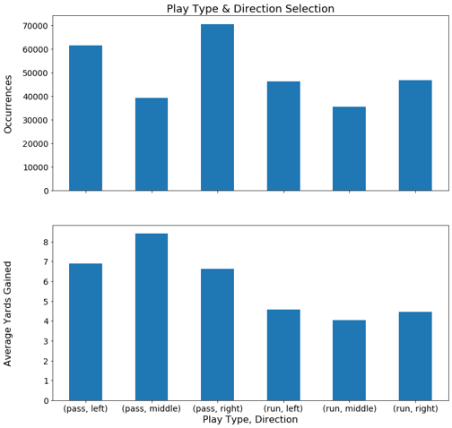
Play calls in the middle (laterally) of the field seem to be the least popular selection. Based on my understanding of the game, I would speculate that this is because the defensive is generally stacked highest in the middle thus running would require going through the greatest number of bodies in this direction and with a pass play there is the least amount of open real estate between defenders to throw the ball in the middle of the field. However, successfully completing a pass in the middle also yields the highest average yards gained. A reason for this could be that catching the ball in the middle of the field leaves a receiver with the largest selection of directions to run after catching the ball.
Team Level Tendencies
An analysis at the team-level granularity could be very useful for a defensive coordinator in that he/she would possess the tendencies of a given team to play the ball in a specific direction and the tendencies for that team to call a run or pass play. This would allow a coordinator to set-up his defensive in schemes as to counteract these tendencies. Table 3 below outlines the percent of plays that are in a specific direction for each given team during the 2018 season.
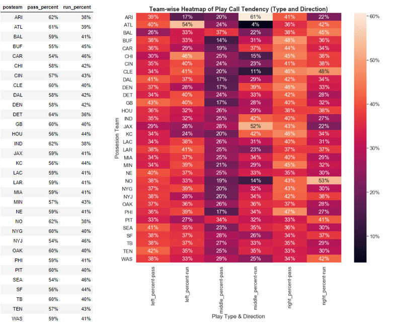
Table 3 and the supporting heatmap can essentially be used as a cheat sheet by both defensive and offensive coordinators. It can be easily updated to account for the latest real-time data. For instance if you are a defensive coordinator and your matchup this week is against the Atlanta Falcons, you can use the table above to understand that they are a pass heavy team (61% pass plays) and they tend to throw the ball to the sides rather than the middle (only 24% of throws in the middle). Furthermore, if you suspect they are going to run on a given play, the table above shows they are highly unlikely to run it down the middle (4% of runs). On the flipside if you are the Atlanta offensive coordinator, you can use this information to more precisely understand how you are spreading the ball and begin to diversify your play call to avoid the traps the defense might be setting up based on your previous tendencies.
Pass vs Run Play Prediction:
Approach
A machine learning application for this dataset is to utilize historical data to try to predict if a specific team is going to call a pass or run play at any given time during a current game. In this case, the problem is formulated to predict pass or run, thus one can attempt to train a binary classification model. After trying a few different approaches ranging from logistic regression to ensemble methods, I settled on a gradient boosted tree model (XGboost) for the final model. In a nutshell, a gradient boosted tree model is chain of decision trees that are trained in a gradual, additive, and sequential manner. Each new tree built tries to improve a bit upon the error propagating from the rest of the chain upstream. There are many resources available online for understanding gradient boosting in more depth and to understand the XGboost package/approach. One such resource is https://towardsdatascience.com/https-medium-com-vishalmorde-xgboost-algorithm-long-she-may-rein-edd9f99be63d.
Model Development & Performance
i) Data subset utilized
To develop this model, data from the 2015-2017 NFL seasons were utilized as the training set while the test set used comprised of the 2018 NFL data. Pre-2015 data was not utilized as rosters, coaching staff, and other evolutions of the team and game occur so frequently that to predict the 2018 season data, it is best to utilize recent season data.
ii) Feature Engineering
The features fed into the model can be found in Figure 7 below. A fair level of data cleaning had to be performed prior to the tendency analysis. Some examples include accounting for team name changes, removing kicking plays, removing extra point plays, removing plays where a penalty occurred, etc. Numerical encoding was performed on categorical features as the XGBoost package utilized does not accept string inputs (but in theory most tree models can accept string inputs). In the feature set, the possession team was label encoded, while the response variable (the “play_type” field) also had to be numerically encoded. Specifically, a 0 represents a run play while a 1 represents a pass play.
iii) Model Tuning
Little model tuning was ultimately performed as a randomized cross-validation grid search showed minimal improvements when testing hyperparameter combinations relative to the defaults in the XGboost python package. Specifically, the random grid search was provided the following parameter ranges:
param_dist = {'n_estimators': [100,200,300],

'learning_rate': [0.01,0.05,0.1,0.5,1.0],

'subsample': [0.3,0.5,0.6,0.7,0.9],

'max_depth': [3,4,5,6,8],

'colsample_bytree': [0.5,0.6,0.7,0.8,0.9],'min_child_weight': [1, 2, 3, 4]}
There are 5 folds fit for 25 different sets of the hyperparameters above resulting 125 total fits. The final model performance is detailed below. Feature importance, for this model is also detailed below. Generally speaking, feature importance provides a score that indicates how useful or valuable each feature was in the construction and predictive capability of the model.


The model achieves a respectable 73% accuracy (with F1 score being in a similar neighborhood) of being able to predict whether a play will be a run or pass play at any given instance of an NFL game. There are some interesting notes from the feature importance plot. The seconds remaining in the half is the strongest parameter followed by the score differential. From domain knowledge, an explanation for this could be that deep field passes are more often seen when the time is running low (in either half) and/or when the possession team is significantly behind in score. Also of interest that the possession team is a strong feature as it supports the notion that studying analytics and tendencies of the opposing team can considerably improve your chances to win by preparing appropriate defensive schemes.
To understand the model’s performance further, the prediction accuracy is further explored by down and yards-to-go combinations. Furthermore a ‘baseline’ prediction accuracy is also provided for comparison. This baseline prediction assumes the more common play type called historically will be called every time in the future for a given combination of down and yards-to-go. E.g. from Table 2, in the case of 1st down and 1-3 yards to go, approximately 70% of the time, a run is called. For the baseline model, when a scenario of 1st down and 1-3 yards to go arises, it will always predict run. This baseline represents the prediction a team would likely make in absence granular statistics like the team-level tendency analysis shown earlier in this document or in absence of advanced analytics such as predictive models.

There are many game scenarios where the baseline prediction is as accurate as the model, but this is mostly in obvious scenarios. For example, the two have similar accuracy in 3rd and long scenarios. This situation is a where the possession team needs more than the average yards gained by running to convert a first down, therefore they are very likely to pass the ball. In scenarios such as 2nd or 3rd down and short where the offense has a wider choice of play selection, the model strongly outperforms the baseline. These less obvious scenarios are exactly where it would help a defensive coordinator to have additional predictive capability or information.
Adding this model to a defensive coordinators toolbelt could provide further information to optimize defensive schemes against any given opponent. Of course, the model could be even more useful if it could predict further details such as the specific type of play that might be called such as a screen play, fly route, sweep to the right, etc. Unfortunately, this level of detailed information was not readily available to parse through. However, based on the data already being collected by the NFL, it is possible this may be available elsewhere.
Player Level Analysis:
This dataset can also allow for analyzing a given player’s impact on a team or game. A quick study performed here is to show how the Denver Broncos offense dramatically improved when they signed Peyton Manning. The three years prior to Peyton joining the team are compared to the three years that he was the starting QB.

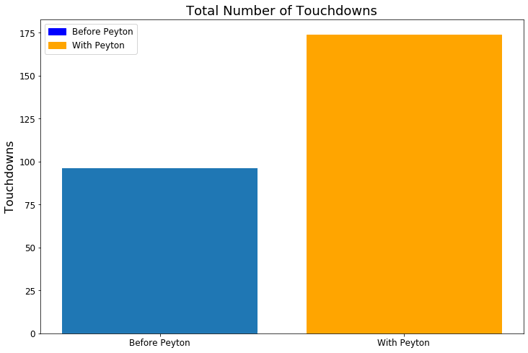
From the above figures, it is clear to see that the Broncos dramatically improved their offensive prowess after adding Peyton Manning to their roster. They gained more yards per game, scored more points per game, and had more possession time per game. This is reflected in their win-loss statistics through these seasons. Namely from 2009-2011 they had 20 wins and 28 losses while from 2012-2014 they had 37 wins and 11 losses.
One might argue that the impact seen is due to numerous factors and not just due to the signing of Peyton Manning. It would be very difficult to separate just his impact to the team’s improved performance, but it is possible to research into some of the potential confounding variables. For instance, a common thought might be that maybe an investment in Peyton also yielded an investment to better the offensive line or wide receivers for the 2012 season.
The O-line remained largely the same between 2011 and 2012, and there was no significant investment into it. However, their performance dramatically changed between the two years. The causal reasoning of this is not explored in detail in this analysis. Something to consider is that the quarterback situation was less defined in 2011 with Tim Tebow and Kyle Orton often splitting the role. Orton is a pocket passer while Tebow rarely stays in the pocket for more than a few seconds. This means the O-line consistently had to adjust its play style. Peyton Manning is a consistent pocket passer and he had sole ownership of the quarterback role in 2012 likely leading to less variability in how the O-line needed to protect the quarterback.
There was also no significant investment in the wide receiver position during Peyton’s first year (additions were made in subsequent years). The most productive wide receivers on the team in 2012 were also on the active roster in 2011 but they were much less productive then. Another consideration is that the coaching staff could have undergone a significant change, however most of the staff including the head coach, the offensive coordinator, and the quarterbacks coach all remained the same between 2011 and 2012.
This analysis shows the potential of utilizing similar and more complex analysis to gauge how player acquisitions/trades are paying off for a given team. More importantly such analyses could dive even deeper to be used to provide insights for salary planning, constructing a team, deploying defensive schemes, and more.
Conclusions:
Performing the analyses contained within this article has served to only deepen my desire to study analytics in the context of the NFL rather than quenching it. The findings from these analyses can provide significant advantage in both offensive and defensive strategies in the NFL. It can help defenses to better prepare and predict their opponents moves while on the flip-side such information can provide visibility to offensives on how they could diversify their play selection. With football being dubbed a ‘game of inches’ the ability to diagnose tendencies with precision or to effectively predict just a few plays could change the course of the entire game. Performing similar analyses with up to date data for a team’s upcoming match would certainty provide a competitive edge that could be the difference in winning or losing. Similar tendency analysis studies extend to baseball, basketball, etc. For example, such analyses are used today to help fine tune defensive shifts in baseball or to determine what aspects of a batters hitting needs to be worked on such that they can counteract such defensive shifts. These types of analytics are being worked on in the field, but it is a relatively new space, especially in the NFL.
The predictive modeling approach and results present a strong use-case in providing more accurate predictions and information to defensive coordinators in difficult game scenarios. The extension of this to the other sports are not as clear as basketball’s more continuous play and baseball’s pitching format do not translate readily into this modeling approach. The player level analysis and use-cases discussed can certainly be extended to almost any other team sport and would likely provide significant value to a general manager and coaching staff.
The analysis performed within this article is just one of many ways to interpret and analyze this type of data. The NFL is acquiring data at a rapid pace and much of this data remains untouched. This document hopes to inspire similar efforts to unlock the potential of this data to help take NFL strategy to the next level.
Continued Work:
There is much more that can be done with the dataset discussed in this article. The model was developed over a very short period and was built with a subset of features manually selected based on domain knowledge. A few suggestions for continued work are:
- Use many more features in the predictive modeling, both those that are readily available in the dataset and others generated through feature engineering. Allow a feature selection approach to select what features are most important.
- Determine if including recent plays called would improve the prediction capability of a model. E.g. use a time-series prediction method such as LSTM or Markov chain approach to model the data
- Collect data on offensive formation (singleback, trips, spread, etc) and perform team level tendency analysis on that as well as adding it as a feature to the predictive model
- Perform analyses to determine what types of plays each team has the most difficulties defending against
- Using the personnel data, an analysis could be performed at the team level to understand what types of plays are called when certain players are on the field.
- Perform a more extensive look into player level analysis to gain insights on optimal building of an NFL team and the associated salary planning
References:
- Morde, V. (2019, April 8). XGBoost Algorithm: Long May She Reign! Retrieved from https://towardsdatascience.com/https-medium-com-vishalmorde-xgboost-algorithm-long-she-may-rein-edd9f99be63d
- Horowitz, M. (2018, December 22). Detailed NFL Play-by-Play Data 2009-2018. Retrieved from https://www.kaggle.com/maxhorowitz/nflplaybyplay2009to2016
- Denver Broncos Team Encyclopedia. (n.d.). Retrieved from https://www.pro-football-reference.com/teams/den/
- Breer, A. (2017, June 27). How Analytics Are Used in the NFL. Retrieved from https://www.si.com/nfl/2017/06/27/nfl-analytics-what-nfl-teams-use-pff-stats-llc-tendencies-player-trac king-injuries-chip-kelly
The code for analysis is located here: https://github.com/pspatel2/nfl_play_by_play_research
Thanks to Max Horowitz for making the scraped play by play data available on publicly on Kaggle. Special thanks also to Borchuluun Yadamsuren, Joel Shapiro, and Finn Qiao for the copyediting and feedback that helped to forge the analysis and write-up into this finished product.